Background
Dazai Osamu (太宰 治) is a 20th-century Japanese novelist. Many of his works centers around mental illness and darkness of human nature, emitting abject or even morbid emotions. His most famous work include Run, Melos! (走れメロス), The Setting Sun, (斜陽) and No Longer Human, (人間失格). He committed suicide in 1948.
The text comes from Aozora Bunko (青空文庫), which is the Japanese Project Gutenberg. I downloaded the txt form of the works, but it is not cleaned as the txt from Project Gutenberg. I have to take out the ruby (inside《》, 笑《わら》う), Japanese pronunciation notation , the notation of the editor (inside[],[#「ファン」に傍点]), and “|” for separation in various conditions.
After cleaning these notation and white space, I first made a character frequency table of Ningen Shikkaku (No Longer Human). I admit I did this manually, chopping the text into single characters and kana, making the frequency table and deleting all kana. If there is a regex expression for kana in R, it will make this work easier.
Here is the first 25 most frequent character in Ningen Shikkaku
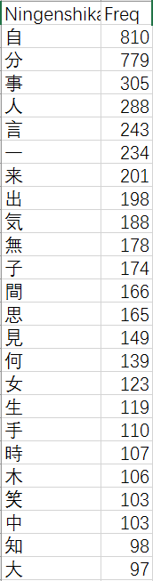
One thing I find intriguing thing about this table is that in such a morbid and hopeless novel like Ningen Shikkaku, Dazai Osamu used the character for laugh (笑) for 103 times, 22nd of all characters. This lead me to look closely into the character and possible vocabularies and conjugations that it forms.
Challenge of Tokenization
The challenge is tokenization. There are many great tools available online, but it takes time to learn to use them, and I do not know if they will work with long text. Therefore, for this week’s text, I used simple code to divide characters and kana into groups of same length. This does not directly solve the problem of tokenization, but rather goes around it.
Here is an example of the code for creating groups of length 2:
g2 <- 2
Text.cleaned.split.group2 <- paste(Text.cleaned.split[1:2], collapse = "")
     for (g2 in 2:(length(Text.cleaned.split) - 1)){
     group2 <- paste(Text.cleaned.split[g2:(g2+1)], collapse = "")
     Text.cleaned.split.group2 <- c(Text.cleaned.split.group2,group2)
}
The code runs so slowly, taking more than 10 seconds for a novel like Ningen Shikkaku. I am going to improve it if I am a better programmer. The same works for grouping of words in length three, four and five, but just runs even slower. For a rough text mining, group of words into length one, two or three should be enough.
The groups with length one, two, three are named
Text.cleaned.split.group1
Text.cleaned.split.group2
Text.cleaned.split.group3
I looked closely into the word formed with laugh (笑). First find every of incidence of character of 笑 in length one.
笑 <- grep(pattern = "笑", Text.cleaned.split.group1)
The start with some initial combination of length two like, 笑う,笑っ, 笑顔, 苦笑, 嘲笑, and find their positions in a vector variable called 笑.two.all. Use setdiff function to find remaining combinations of length two, adding them to my list. Here is an example:
笑う <- grep(pattern = "笑う", Text.cleaned.split.group2)
笑っ <- grep(pattern = "笑っ", Text.cleaned.split.group2)
笑顔 <- grep(pattern = "笑顔", Text.cleaned.split.group2)
嘲笑 <- grep(pattern = "嘲笑", Text.cleaned.split.group2) + 1L
笑.two.all <- c(笑う,笑っ,嘲笑,笑顔)
笑.others <- setdiff(笑,笑.two.all)
At the end, I come up with a list of 21 possible combinations in 16 works of Dazai Osamu :
笑う,笑い,笑っ,笑わ,笑む,笑声,失笑,笑ん,笑話,微笑,嘲笑,苦笑,笑顔,媚笑,可笑,一笑,の笑,笑え,憫笑,叟笑,笑お
When an author use the word laugh (笑), it is not always a positive word. We can have smile (微笑), and laughing face (笑顔), but we also have to laugh at (嘲笑) and bitter laugh (苦笑).
Analyzing: positive or negative
My idea is to roughly group the combinations of length 2 into positive and negative laugh.
笑.two.positive <- c(笑う,笑い,笑っ,笑む,笑声,失笑,笑ん,微笑,笑顔,笑話,一笑,笑え,叟笑,笑お)
笑.two.negative <- c(笑わ,嘲笑,苦笑,媚笑,憫笑)
I then did a word frequency bar graph of the positive and negative laughter in all 16 works of Dazai Osamu. I put them all in chronological order, because I want to find if there is a change in style of the use of word.
ggplot(Freq.novel.df,aes(x = reorder(type,-value), y= value, fill = color))+
 geom_bar(stat="identity",color="grey50",position = "dodge", width = 1) +
 xlab("Type") + ylab("") +
 scale_fill_manual(values=c("dodgerblue2","firebrick3"),guide = FALSE) +
 ggtitle("1948_6_Ningenshikkaku")
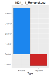
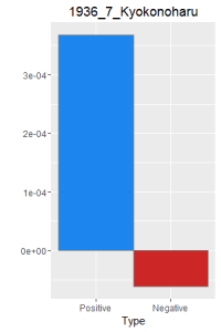
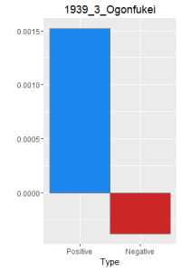
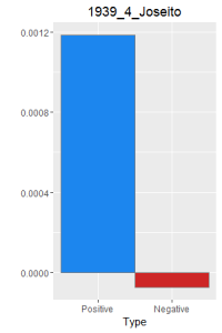
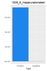
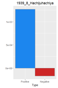
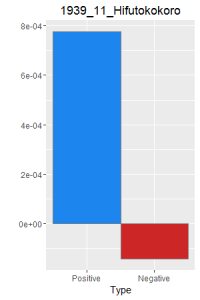
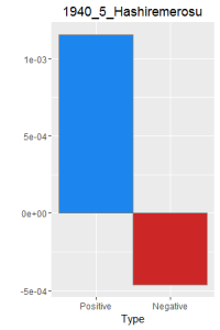
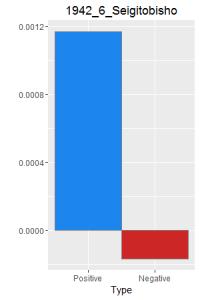
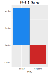
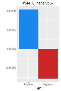
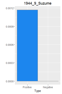
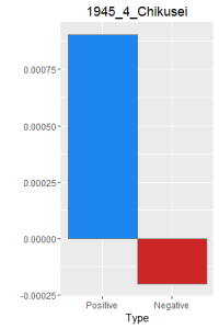
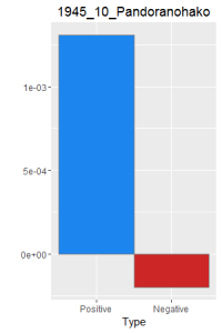
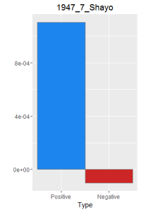

After making this graphs I find that short stories are more likely to become outliers, because they do not use the word a lot. Here is a comparison of the four novels. As I expected, Ningen Shikkaku is the has the most negative use of laugh.
Reflection
I can make more graphs with my data from this week. For example a scattor plot of line plot with a x-axis in chronological order. Refining my searching lexicon can provide better data.
I can also search for place names with words with my group2, since most place names are in two characters. If I try to map it, I expect to get an enormous cluster around cities like Tokyo.
Doing text mining in languages like Japanese is hard, but not impossible. The method that I used in this week’s post will become tedious as I refine my searching lexicon. I can, however, run the same code on as many texts as I want, if my laptop does not crash because the verbosity of my code.
Full code:
library(stringr)
library(ggplot2)
Read in the file
Text.df <- read.delim("D:/Google Drive/JPN_LIT/Dasai_Osamu/1948_6_Ningenshikkaku.txt", header = FALSE, stringsAsFactors = FALSE, encoding = "CP932")
Text.text <- paste(Text.df[,1],collapse = "")
Text.splited.raw <- unlist(str_split(Text.text, pattern = ""))
Text.splited <- str_replace_all(Text.splited.raw, "|", "") # Take out all "|"
###grep
## Take out ruby and style notation
# Find out where to start and end
start <- grep(pattern = "《|[", Text.splited)
end <- grep(pattern = "》|]", Text.splited)
from <- end + 1
to <- start - 1
real.from <- c(1, from)
real.to <- c(to, length(Text.splited))
CUT.df <- data.frame("from" = real.from, "to"= real.to,"text" = NA)
# Solve the situation when form > end
row <- 1
CUT.fine.df <- data.frame("from" = 0, "to" = 0, "text" = NA)
for(row in 1:length(CUT.df$from)){
 if(CUT.df$from[row] <= CUT.df$to[row]){
 CUT.fine.df<- rbind(CUT.fine.df, CUT.df[row,])
 }
}
i <- 1
for(i in 1:length(CUT.fine.df$from)){
 text <- Text.splited[CUT.fine.df$from[i]:CUT.fine.df$to[i]]
 CUT.fine.df$text[i] <- paste(text, collapse = "")
}
Text.cleaned.text <- paste(CUT.fine.df$text, collapse = "") #cleaned up text, without ruby and style notations.
Text.cleaned.split <- unlist(str_split(Text.cleaned.text, pattern = ""))
###Run Code if you want a cleaned txt of the text
###Change name if needed
# write.table(Text.cleaned.text,"shayo.txt",row.names = FALSE, col.names = FALSE)
## A simple word count here (All punctuation, white spaces in English or Japanese format)
Text.wordcount <- str_replace_all(Text.cleaned.split, "[:punct:]", " ")
Text.wordcount <- Text.wordcount[which(Text.wordcount != " ")]
Text.wordcount <- Text.wordcount[which(Text.wordcount != " ")]
Text.freq <- data.frame(table(Text.wordcount))
Text.freq.ord <- Text.freq[order(-Text.freq$Freq),]
### Run code if you want a wordcount table.
### Change name if needed
write.table(Text.freq.ord, "Shayo_freq.txt",row.names = FALSE, sep = "\t")
### Grouping according to character length
## Runs slowly.
## Do not use unless necessary. Uncomment before use.
Text.cleaned.split.group1 <- Text.cleaned.split
g2 <- 2
Text.cleaned.split.group2 <- paste(Text.cleaned.split[1:2], collapse = "")
for (g2 in 2:(length(Text.cleaned.split) - 1)){
 group2 <- paste(Text.cleaned.split[g2:(g2+1)], collapse = "")
 Text.cleaned.split.group2 <- c(Text.cleaned.split.group2,group2)
}
# g3 <- 2
# Text.cleaned.split.group3 <- paste(Text.cleaned.split[1:3], collapse = "")
# for (g3 in 2:(length(Text.cleaned.split) - 2)){
# group3 <- paste(Text.cleaned.split[g3:(g3+2)], collapse = "")
# Text.cleaned.split.group3 <- c(Text.cleaned.split.group3,group3)
# }
#
# g4 <- 2
# Text.cleaned.split.group4 <- paste(Text.cleaned.split[1:4], collapse = "")
# for (g4 in 2:(length(Text.cleaned.split) - 3)){
# group4 <- paste(Text.cleaned.split[g4:(g4+3)], collapse = "")
# Text.cleaned.split.group4 <- c(Text.cleaned.split.group4,group4)
# }
#Word with length one
笑 <- grep(pattern = "笑", Text.cleaned.split.group1)
#Word with length two
笑う <- grep(pattern = "笑う", Text.cleaned.split.group2)
笑い <- grep(pattern = "笑い", Text.cleaned.split.group2)
笑っ <- grep(pattern = "笑っ", Text.cleaned.split.group2)
笑わ <- grep(pattern = "笑わ", Text.cleaned.split.group2)
笑え <- grep(pattern = "笑え", Text.cleaned.split.group2)
笑お <- grep(pattern = "笑お", Text.cleaned.split.group2)
笑む <- grep(pattern = "笑む", Text.cleaned.split.group2)
笑ん <- grep(pattern = "笑ん", Text.cleaned.split.group2)
笑顔 <- grep(pattern = "笑顔", Text.cleaned.split.group2)
笑話 <- grep(pattern = "笑話", Text.cleaned.split.group2)
笑声 <- grep(pattern = "笑声", Text.cleaned.split.group2)
微笑 <- grep(pattern = "微笑", Text.cleaned.split.group2) + 1L
嘲笑 <- grep(pattern = "嘲笑", Text.cleaned.split.group2) + 1L
苦笑 <- grep(pattern = "苦笑", Text.cleaned.split.group2) + 1L
媚笑 <- grep(pattern = "媚笑", Text.cleaned.split.group2) + 1L
可笑 <- grep(pattern = "可笑", Text.cleaned.split.group2) + 1L
一笑 <- grep(pattern = "一笑", Text.cleaned.split.group2) + 1L
憫笑 <- grep(pattern = "憫笑", Text.cleaned.split.group2) + 1L
叟笑 <- grep(pattern = "叟笑", Text.cleaned.split.group2) + 1L # For北叟笑む
失笑 <- grep(pattern = "失笑", Text.cleaned.split.group2) + 1L
の笑 <- grep(pattern = "一笑", Text.cleaned.split.group2) + 1L # This is the case when 笑 stands alone
# #Word with length three (uncomment before use)
# 笑われ <- grep(pattern = "笑われ", Text.cleaned.split.group3)
# 笑わせ <- grep(pattern = "笑わせ", Text.cleaned.split.group3)
#
# #Word with length four(uncomment before use)
# 笑いませ <- grep(pattern = "笑いませ", Text.cleaned.split.group4)
笑.two.all <- c(笑う,笑い,笑っ,笑わ,笑む,笑声,失笑,笑ん,笑話,微笑,嘲笑,苦笑,笑顔,媚笑,可笑,一笑,の笑,笑え,憫笑,叟笑,笑お)
笑.two.positive <- c(笑う,笑い,笑っ,笑む,笑声,失笑,笑ん,微笑,笑顔,笑話,一笑,笑え,叟笑,笑お)
笑.two.negative <- c(笑わ,嘲笑,苦笑,媚笑,憫笑)
笑.two.neutral <- c(可笑,の笑)
笑.others <- setdiff(笑,笑.two.all)
##### Graph Section of the code
###笑 divided positive and negative as frequecy in the novel
postive.freq <- length(笑.two.positive) / length(Text.wordcount)
negative.freq <- - length(笑.two.negative) / length(Text.wordcount)
Freq.novel.df <- data.frame ("type"= c("Positive", "Negative"), "value" = c(postive.freq,negative.freq),color = c("1","2"))
Freq.novel.df$type <- as.character(Freq.novel.df$type)
ggplot(Freq.novel.df,aes(x = reorder(type,-value), y= value, fill = color))+
 geom_bar(stat="identity",color="grey50",position = "dodge", width = 1) +
 xlab("Type") + ylab("") +
 scale_fill_manual(values=c("dodgerblue2","firebrick3"),guide = FALSE) +
 ggtitle("1948_6_Ningenshikkaku")