The fundamental unit of the brain is the neuron, and the computational essence of a neuron is adding up blips from neurons it listens to then “deciding” whether to issue a blip to neurons that listen to it. Perhaps the simplest representation of the computational neuron is the so-called leaky integrate and fire model, which adds up a smoothed out version of the incoming blips (the integrate part), subtracts off a bit if the blip came farther in the past (the leaky part), then transmits a blip of its own if the sum breaches a pre-set threshold (the firing part). [Download the simple LIF simulator.]
The leaky integrate and fire (LIF) model captures the bare minimum neuron physiology required for its basic computational purpose. The “blips” are boluses of electric charge (action potentials) traveling down the neuron’s body like a wire. The integration of blips is physically executed in the neuron by an accumulation of voltage resulting from all the incoming electric charge blips. The neuron naturally leaks out some of the charge as its adding up all the blips because it isn’t perfectly insulated from the body. To issue an outgoing blip tiny pores in the neuron orchestrate a careful balance of opening and closing to let out a short burst of charge down its body that is connected to a host of other neurons listening for such blips.
It is common to use LIF neurons as an introduction to studying how the nervous system computes things because, according to Einstein (maybe), a scientific theory should be as simple as possible, but no simpler. The LIF model prunes away all the messy neuroscience leaving only the neuron’s core information processing machinery: temporally integrate incoming action potentials to trigger one of its own. Connect LIF neurons together, and we can build basic circuits.
I wrote SimLIFNet for MATLAB as the simplest possible tool for getting started with networks of the simplest possible neurons: in two lines you can 1) define which neuron is connected to which others, then 2) simulate the network.
>> Get the code, which is a single m-file, here: Easily Simulate Custom Networks of LIF Neurons
The function can run simple, out-of-the box networks or more customized setups that let you set numerical integration time steps, refractory periods, forcing functions, noise, synaptic densities, and other common parameters. Examples are provided from a pair simple interacting neurons to networks that compute logical operations.
Take this simple example of two neurons negatively connected to each other (inhibition), with one getting continuous external activation.
W = [ 0.0 -0.2; -0.2  0.0];
spkFull = SimLIFNet(W,'offsetCurrents',[1.1; 0]);
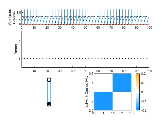
From the two lines, SimLIFNet generates plots of each neuron’s membrane potential (top), the time action potentials were fired (middle), a schematic diagram of the network (bottom left), and a heatmap of the connectivity matrix (lower right).
The networks can get as complicated as you like. Hopefully this is a useful tool for anyone building up their intuitions for how simple neural circuits work to compute. Happy spiking!
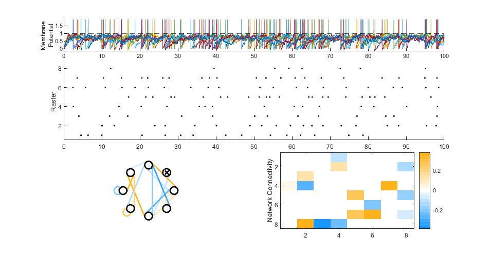
W = 1*rand(8)-0.5;
W(randperm(numel(W))>round(0.25*numel(W))) = 0;
[spk, NetParams, V] = SimLIFNet(W,'simTime',100,'tstep',1e-2,...
     'offsetCurrents',0.8*ones(length(W),1),...
     'noiseAmplitude',0.2*ones(length(W),1));