Softmax is supposed to be a function that will tell you, given a list of measurable features about an example (e.g. how red is the picture, how tall is the plant, how many bedrooms does the structure have), how likely it is to belong to a certain group (e.g. it’s a firetruck, it’s a sunflower, it’s a townhouse). Softmax takes in a list of numbers indicating “how much” of each feature an example has and gives back a list of numbers indicating how likely it is the example belongs to each group. (This process is essentially identical to multinomial logistic regression, for anyone keeping score, but we call it Softmax when the function is at the end of an artificial neural network.) But it’s hard for me to square what Softmax is actually doing with the interpretation we are ostensibly asked to glean from its outputs.
What is Softmax
To define Softmax we can say that given an input example, x, and the model, A, our estimate of the probability that the input belongs to each potential group, g, is calculated as:
![]()
Each element of the input example, x, is a list of numbers of how much the example has of each feature. Each element of the output, g, is a list of numbers between 0 and 1 indicating the probability the example belongs to each group (or class). The model, A, is determined by regression, that is, given many examples that are labeled with their correct group we can numerically find some set of numbers in A that makes Softmax give back the correct groups when we feed in all the labeled examples. We then hope that it works well on new examples also, which is how regression generally works.
Wait, What is Linear Regression Again?
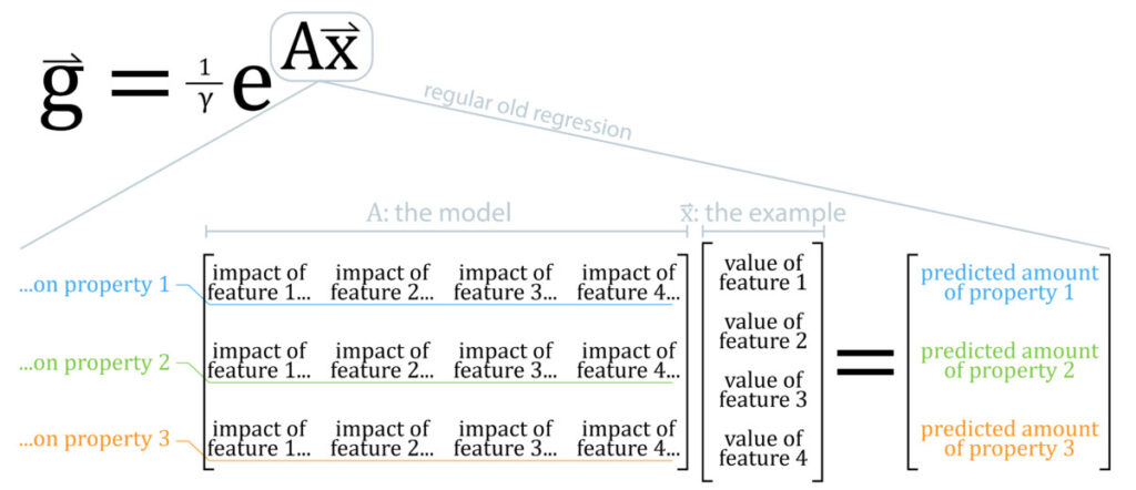
The main thing to notice is that Softmax looks an awful lot like regular old regression, Ax, just pushed up into the exponent of e. (In fact, generalized versions of linear regression follow this logic, where we put linear regression inside another (link) function.) So, let’s quickly examine regular old regression.

In regular old regression we predict how much of each property a given input example will have based on the the values of the input example’s features. The matrix A, our model, is what specifies exactly how much the features of the example contribute to its predicted properties.
A particular house, x, might have 3 bedrooms (feature 1), 1.5 baths (feature 2), 1800 sqft. (feature 3), and be 2 miles from the highway (feature 4). We weigh the values of these features with A to predict how many dollars the house will sell for (property 1), in how many days the house will sell (property 2), and how many buyers will view it prior to the sale (property 3).
The point is that the model predicts HOW MUCH of each property an example will have given the value of its features.
Linear Regression in an Exponent
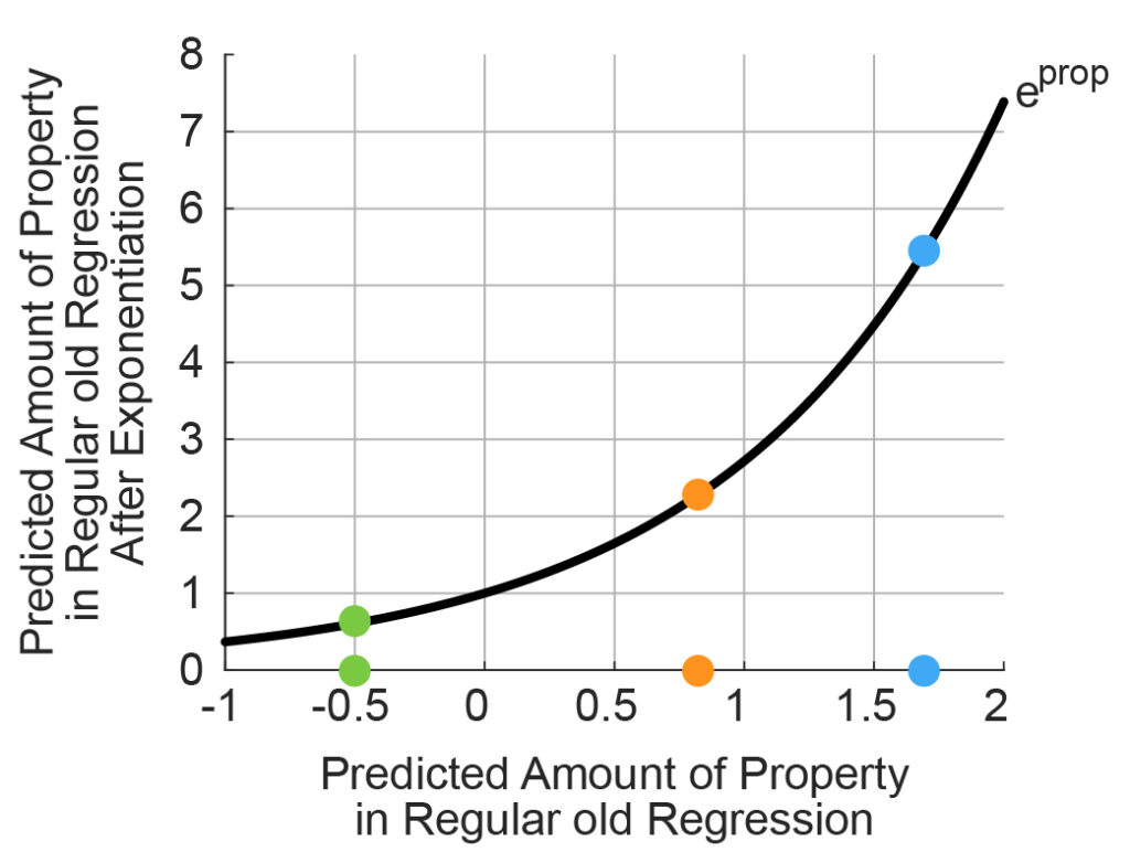
What happens when we put this model in the exponent of e?
Properties we predicted were less than zero all get squished to the interval between 0 and 1 (the green property -0.5=>~0.6), while properties we predicted were large and positive get enormous (orange ~0.8=>2.2, blue ~1.7=>~5.4).

This quality of modest becoming large and large becoming enormous is where Softmax gets its name; if any one property is predicted to be even somewhat larger than the others by regular old regression, Softmax makes that larger property totally dominate the others via exponentiation. It isn’t exactly a max function because the other properties aren’t exactly zero (and so we are supposed to interpret that to mean there is a non-zero chance they have that property or belong to that group), but they are all pretty close to zero compared to the (usually) one dominant property. Thus, it isn’t a hard-max, its a Softmax.
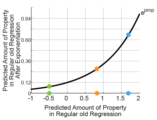
The normalization factor we are dividing by doesn’t change this story (1/gamma), it is simply chosen to scale all the amounts of each predicted property so they all sum to 1, but their relative differences are not affected (figure below). Normalization does have the nice attribute of ensuring the largest predicted property value does not exceed 1, so one can define various thresholds on these property predictions that easily translate to many contexts. Since all predictions add to 1, and none are negative, it is also technically a discrete probability distribution (think of a fair 6-sided die where each outcome has 1/6 probability).

Interpreting Softmax Outputs
Consolidating the discussion, regular old regression predicts the amount of various properties an example has given a list of how much of each feature the example has. For Softmax, we then exponentiate that regression process, making the largest predicted property value much larger than the others (then making sure all predicted property values sum to 1).
How should we then understand the Softmax outputs? In practice, people mentally assign each element in the output as the corresponding probability the example belongs to that group. If Softmax outputs 10 values, it is supposed that each value is the predicted chance that the input belongs to each of the 10 groups, and that we are justified in thinking this way because all the output values for any example sum to 1, just like a discrete probability distribution.
But, if we take the classic interpretation of regular old linear regression seriously, then each Softmax output corresponds to how much of a given property we predict our input example has. If we mentally assign each Softmax output to a group, rather than a typical feature (like sale price of a house), the 1st output appears to actually represent “how much group 1 we predict for this example”, and the 2nd “how much group 2 we predict for this example”. This phrasing is perhaps awkward, but is a direct extension of what the world has agreed that regular old regression means. The fact that we exponentiate the regression doesn’t fundamentally change its meaning.
For me, phrasing Softmax outputs like this, “how much group N do we predict for this example”, helps me to not take Softmax output so seriously. The function we put our regular old regression into could really be anything. So long as we have some way to rank order the outputs of regular old regression or quantify the relative difference in magnitude of the outputs we can build the same type of model, one that predicts which group a given example belongs to.
One could easily imagine all sorts of nearly equivalent variations.
![]()
You might recognize the above as the classic deep learning ReLU function – just normalized. Why not? We get a discrete probability distribution on our outputs, after all.
Even something as crazy as the following could work:
![]()
Where I mean simply squaring the output of the regression. This would count both very positive predictions, “lots of group N”, and negative predictions, “lots of negative group N” toward the likelihood of being in that given group. It’s essentially interpreting the regression as saying we are unlikely to be in a given group only when the prediction is near zero. Any increase in magnitude, positive or negative, increases the likelihood of classifying the example as being in the given group. Why not? Maybe it’s useful for predicting a person’s position on a political issue, given the horseshoe politics theory.
Even some of the AI greats have taken liberties with Softmax, introducing a new term in the exponent to control how much the exponentiation exaggerates the largest predicted property value relative to the rest. They call the parameter “temperature”. Changing the temperature is an easy way to make model predictions a bit more spontaneous, which is useful to make LLMs more relatable (they get pretty boring when they always choose the most likely next word instead of mixing it up more often).
Conclusions
There’s nothing sacred about Softmax. Its outputs are more like, “how much group-1-ishness” do I predict this example has than, as is the typical interpretation, the probability it belongs to that group. Recognizing this should set you free. Experiment will all sorts of rank order functions and output rescalings. Even the requirement to have the outputs sum to 1 isn’t strictly required, it’s just there to help make choosing a final winner from among all the outputs simpler and more generalizable. This advice doesn’t necessarily hold if you are working in the rigorous space of proving things about statistics, since Softmax does have a special form among the exponential family of distributions that guarantees it some important properties, but deep learning has been playing fast and loose with rigorous mathematical underpinnings for years. Go experiment. Knock yourself out.
