Author: Tarushi Tanaya

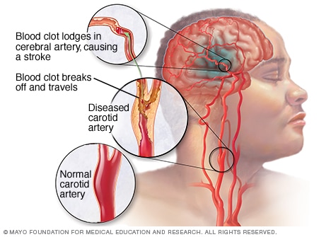
In lab, I have generated a protocol (as seen below)  to operate within a neural-imaging software called LCModel. So far the process has been long and arduous, with not much usable data being collected due to shims, or faulty MRI scanning procedures. Most of my analysis will likely be methodolgically based as opposed to being grounded in emprical data. Despite this, the following protocol may prove useful as tool to help troubleshoot with errors that may appear in LCModel. Using Terminal, one can use the protocol to run LCModel in order to analyze their spectral data.

How to tunnel

• Open Terminal>input: ssh -Y username> enter password
• Ls to check if in the right place
• cd CABI_MRS
• Matlab &
• All output goes to ‘Documents>CABIStroke>GABA>GABA processing sheet’

How to find PW

• “Keychain”> Show bitc password> PW 2x> Copy and Paste PW into terminal

PREPROCESSING

• In Terminal:
  • “matlab &” opens MATLAB
• In MATLAB:
  • Open MATLAB>scripts>readSiemens_stability_CABI_MRS.m
• Change path where it says inDir line 9 and outDir line 10
  • Go to Fetch to check file pathway
  • Example inDir: ‘/home/michael.borich/CABI_MRS/SS_###/#T_CMRRR_GABA_10min_1#
  • Example outDir: ‘/home/michael.borich/CABI_MRS/Processed/SS_###/#T
  • Make sure line 12 has the spectral_reg_flag set to 1 as default
• Figure 2:
  • Baseline must be as straight and as close to zero as possible, adjust phase change value if it is not so.
    • If you want to change phase value, hit “y” when prompted. If not, hit “n”
    • Change phase value “y”>-10<x<10 (approx.)> if sufficient, “n”
  • Enter phase change value in GABA processing spreadsheet (column B)
• Figure 1:
  • Blue and red peaks should both be symmetrical around 3 ppm
  • To change freq value if necessary enter “y” as prompted and then enter appropriate no.
  •  Enter freq change value in GABA processing spreadsheet (column C)
• Figure 3:
  • Enter “n” (will not need to change phase value)
• Figure 4:
  • Click before and after peak
  • Outputs with fullwidth_Hz_H20
  • Enter value in GABA processing spreadsheet (column D)
• Figure 5:
  • Click before and after peak
  • Outputs with fullwidth_Hz_NAA
  • Enter value in GABA processing spreadsheet (column E)
• Figure 6:
  • Click before and after peak around 3 ppm (creatine peak)
  • Outputs with fullwidth_Hz_Cr
  • Enter value in GABA processing spreadsheet (column F)
  • Value should ideally be less than 12

• To obtain GABA.water file
  • In Terminal:
    • “matlab &” opens MATLAB
  • In MATLAB:
    • Open MATLAB>scripts>readSiemens_GABA_water.m
  • Change path where it says inDir line 9 and outDir line 10
    • Go to Fetch to check file pathway
    • Example inDir: ‘/home/michael.borich/CABI_MRS/SS_###/#T_CMRRR_GABA_10min_1#
    • Example outDir: ‘/home/michael.borich/CABI_MRS/Processed/SS_###/#T

• Errors:
  • If error comes up that mentions nlinfit, go to line 12> change =1 to =0
    • “save”>”run”> enter new phase change value
  • If Diagnostics are Red then google how to check for error
  • If error comes up that mentions line 181

PROCESSING

Open LCModel

•  Open terminal>[keep spaces]ssh -Y node7
• Enter password
• Open LCModel:
  • cd ~/.lcmodel
  • ./lcmgui &
• “Select User Profile” window will appear, select “GABA”
• “Select your data type” window will appear, select “Other”

• Loading the DIFF data into LCModel
  • Follow path: home/michael.borich/CABI_MRS/Processed/SS_###/#T/DIFF*
    • Select “GABA.raw”
  • “Control Parameters” window appears
    • Select “Change BASIS”
    • Select file that ends in “_DIFF.basis”
  • Add “DIFF” to the end of output file path (next to Reconfigure button)
  • Click “Advanced Settings”
    • Click “Change Control-Defaults file” and make sure “GABA_DIFF” is selected
  • HIT Run LCModel
  • You will be prompted to select UNSUPPRESSED Water Reference RAW file
    • Select “GABA_water.raw”
  • Graphic should appear
    • Red line=model
    • Black line= raw data
    • Two lines should have as much overlap as possible
  • Record Data on the spreadsheet>
• Loading the OFF data into LCModel
  • Follow path: home/michael.borich/CABI_MRS/Processed/SS_###/#T/OFF*
    • Select “GABA_off.raw”
  • “Control Parameters” window appears
    • Select “Change BASIS”
    • Select file that ends in “_OFF.basis”
  • Add “OFF” to the end of output file path (next to Reconfigure button)
  • Click “Advanced Settings”
    • Click “Change Control-Defaults file” and make sure “GABA_OFF” is selected
  • HIT Run LCModel
  • You will be prompted to select UNSUPPRESSED Water Reference RAW file
    • Select “GABA_water.raw”
  • Graphic should appear
    • Red line=model
    • Black line= raw data
    • Two lines should have as much overlap as possible

 

An Introduction to Freesurfer

Freesurfer is a processing software commonly used for the purposes of neuroimaging processing and data analysis. It allows for the visualization of structural and functional areas of the brain, making it especially useful in my field of research, which explores the role of Gamma Amino Butyric Acid (GABA) as a biomarker in the prognosis and treatment trajectories in stroke patients. Processing through the Freesurfer pipeline is conducted through C shell, a Terminal shell which is used as an executive command interpreter.

This blog post is meant to document some of the procedural aspects of data analysis in my subset of neuroscience research, which mainly includes neuroimaging and topographical mapping of the brains of patients who have suffered from stroke. As an undergraduate, I have relatively little experience writing scripts and computer programming; this post is meant to be a guide to beginners on how to I utilized the Freesurfer pipeline as I peruse and attempt to solve the methodological complications that may arise while creating and editing scripts within the pipeline myself.

 

Methods and Directives I have Completed thus Far:

$Autoreconall-1, $Autoreconall-2, and $Autocreconall-3, are all a series of commands used in the reconstruction of cortical images based on post-stroke T1 MRI scans of patients. These co

mmands scan for topographical errors and are known as clustered directives. Clustered directives allowed me to perform a series of commands all at once, thus more efficient processing and correcting brain scans. Additionally commands such as $foreach allow one to process the scans for each subject all at once, thus minimizing the amount of script I had to input into Terminal, the MAC operating system that hosts C shell.

 

The processing of these images took about three days to complete, and one subject had to be thrown out due to an excess of topographical images found on the original T1 MRI. After these were complete, I was able to utilize Freeview, a visualization tool within the Freesurfer pipeline, to look at the final, reprocessed brain volumes and check for any abnormalities, such as whether regions of the brain were cutoff. An example of a sample scan visualized in Freeview can be seen below:

Finally after this has been completed, a stats script was used in order to extract statistical data. However, after attempting to input the script an error (shown in the image below) came up. Although, according to others working within C shell or BASH, this seems to be a fairly common error, none of the suggested corrections to the script (most of which came from this thread: https://askubuntu.com/questions/304999/not-able-to-execute-a-sh-file-bin-bashm-bad-interpreter) seemed to help resolve the issue.  Hopefully these will be resolved within the week.

/bin/bash^M: bad interpreter: No such file or directory

What is Stroke?

Stroke is the leading cause of disability in the United States. The condition causes rapid plasticity within various cortical connections in the brain, essentially causing a remap of neural circuiting in affected areas. When remapping occurs, it forces area of the cortex to form new connections, also known as long-term potentiation. This diminishes responsiveness in certain areas of the brain. In human stroke patients, the damage manifests itself in decreased language, motor, and sensory transfers of information caused by changes in neuronal excitation, which are primarily localized in the somatosensory and primary motor cortices of the brain. ^1,2

The heterogeneity of stroke can make it difficult to diagnose, determine prognosis trajectories, and determine an appropriate treatment plan, making the identification of biomarkers⁸ an imperative tool to determine the level of changes in neural circuitry. However, as far as current research goes, there are no established biomarkers for stroke patients, especially within the context of hemodynamic and neurochemical activity. Whole brain analysis provides significant evidence to suggest a negatively correlative relationship of GABA localized within the primary motor cortex⁹, indicating that GABA may be a viable biomarker for stroke.¹ Additionally, multiple studies have linked decreased levels of GABA in the primary cortex after various non-invasive brain stimulation techniques (NIBS).^1,5,8,10

What has previous research shown?

In previous studies, NIBS and PETs techniques were used in order to monitor and record GABAergic activity, however, these do not measure GABA levels directly.¹ Magnetic resonance spectroscopy (MRS) has been useful non-invasive techniques have been useful in measuring GABAergic synaptic activity.⁷ Magnetic resonance imaging (fMRI) performed at baseline and after NIBS patients show that decreases in GABA are associated with motor recovery in chronic settings as well.¹ While the relationship is between GABA and motor learning is apparent, further research is necessary on how total concentrations GABA within larger volumes of cortical tissue relate to the synaptic activity¹⁰, and establish which mechanisms decrease GABA and are responsible for neural remapping.⁸

Identifying Biomarkers

Pairing NIBS with MRS and fMRI addresses many technical problems associated with using the techniques separately. Data are collected at the same point in time, rather separately, increasing reliability and strengthening the relationship between NIBS techniques and changes before, during, and after interventions². fMRI-MRS techniques are shown to provide information on neural activity and neurochemical concentrations of various brain states, respectively.⁴ Physiological and cognitive variables are then easier to identify, and support link between the motor cortex and its chemical milieu.⁶ This comparability is especially important when trying to link hemodynamic and neurochemical responses, the former of which ceases after prolonged periods of stimulation. ⁴

What does this help us understand?

This research should help inform future rehabilitative techniques that aim to promote neural plasticity and at least partial restoration of motor functioning in post-stroke patients and assist in the stratification of patient treatment and help isolate which behavioral changes and interventions will most benefit any given patient⁸, in addition to determining the neuro-metabolic mechanisms responsible for learning, regaining motor-functioning, and specific for task encoding.³

References

1. Blicher, J., Near, J., Næss-Schmidt, E., Stagg, C., Johansen-Berg, H., & Nielsen, J. et al. (2014). GABA Levels Are Decreased After Stroke and GABA Changes During Rehabilitation Correlate With Motor Improvement. Neurorehabilitation And Neural Repair, 29(3), 278-286. http://dx.doi.org/10.1177/1545968314543652
2. Carmichael, S. (2012). Brain Excitability in Stroke. Archives Of Neurology, 69(2), 161. http://dx.doi.org/10.1001/archneurol.2011.1175
3. Floyer-Lea, A. (2006). Rapid Modulation of GABA Concentration in Human Sensorimotor Cortex During Motor Learning. Journal Of Neurophysiology, 95(3), 1639-1644. http://dx.doi.org/10.1152/jn.00346.2005
4. Ip, I., Berrington, A., Hess, A., Parker, A., Emir, U., & Bridge, H. (2017). Combined fMRI-MRS acquires simultaneous glutamate and BOLD-fMRI signals in the human brain. Neuroimage, 155, 113-119. http://dx.doi.org/10.1016/j.neuroimage.2017.04.030
5. Koch, G., Ponzo, V., Di Lorenzo, F., Caltagirone, C., & Veniero, D. (2013). Hebbian and Anti-Hebbian Spike-Timing-Dependent Plasticity of Human Cortico-Cortical Connections. Journal Of Neuroscience, 33(23), 9725-9733. http://dx.doi.org/10.1523/jneurosci.4988-12.2013
6. Kolasinski, J., Logan, J., Hinson, E., Manners, D., Divanbeighi Zand, A., & Makin, T. et al. (2017). A Mechanistic Link from GABA to Cortical Architecture and Perception. Current Biology, 27(11), 1685-1691.e3. http://dx.doi.org/10.1016/j.cub.2017.04.055
7. Mullins, P., McGonigle, D., O’Gorman, R., Puts, N., Vidyasagar, R., Evans, C., & Edden, R. (2014). Current practice in the use of MEGA-PRESS spectroscopy for the detection of GABA. Neuroimage, 86, 43-52. http://dx.doi.org/10.1016/j.neuroimage.2012.12.004
8. Sato, S., Bergmann, T., & Borich, M. (2015). Opportunities for concurrent transcranial magnetic stimulation and electroencephalography to characterize cortical activity in stroke. Frontiers In Human Neuroscience, 9. http://dx.doi.org/10.3389/fnhum.2015.00250
9. Stagg, C. (2014). Magnetic Resonance Spectroscopy as a tool to study the role of GABA in motor-cortical plasticity. Neuroimage, 86, 19-27. http://dx.doi.org/10.1016/j.neuroimage.2013.01.009
10. Stagg, C., Bestmann, S., Constantinescu, A., Moreno Moreno, L., Allman, C., & Mekle, R. et al. (2011). Relationship between physiological measures of excitability and levels of glutamate and GABA in the human motor cortex. The Journal Of Physiology, 589(23), 5845-5855. http://dx.doi.org/10.1113/jphysiol.2011.216978