In fall 2014 I taught a freshman seminar on data visualization entitled “Charts, Maps, and Graphs.” Over the course of the semester I worked with the students to create vizs that passed Tukey’s “intra-ocular trauma” test: the results should hit you between the eyes. Over the coming months I’ll be blogging based on their final projects.
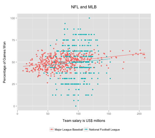
Today’s post is based on the work of Jeffrey You, who used US professional sports data, comparing baseball and football. As Jeffrey noted, the vizs highlight two key differences between the sports. First, the shorter football season (16 vs. 162 games per season) means that many football teams finish with the same record. The NFL scatterplot is therefore striated, and the winning percentage looks like a discrete variable. In fact there are limited outcomes for both baseball and football, but 162 possibilities looks continuous while 16 does not.
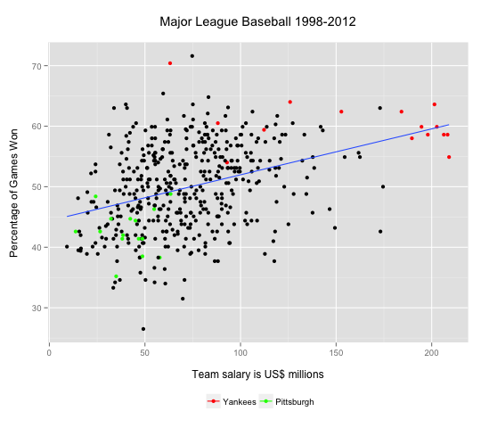
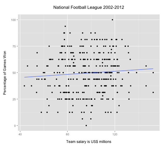
The other contrast is relative importance of total payroll in baseball. In neither case is there a strong correlation, but football is astonishingly low: r= 0.07 for the NFL compared to r=0.37 for MLB. What’s going on? Jeffrey suspected that injuries might play a greater role in the NFL, so a high payroll might pay for less actual playing time. He noted as well, the greater importance of single player. Tom Brady, he noted, was a 199th draft pick with a starting salary of “only” $375,000.
The graphs also highlight the greater payroll range in MLB compared to the NFL. The regression line for MLB suggests that increasing a win-loss record by one game costs about $8 million. But the payroll spread in MLB so large that it can become a dominant factor. Jeffrey noted that for 2002-2012 the average payroll for the Yankees was $162 million while that of the Pirates was merely $41 million. For that same period, the Yankees have never won less than 50% of their games while the Pirates never won more than 50%. There is no comparable phenomenon for football. The standard deviation for MLB payrolls is about $35 million but for the NFL it’s less than $20 million.
NB: Technically, one should use the log of the odds rather than use winning percentage as the dependent variable, but in this case the substantive results are the same. For MLB the values range from 25% to 75%, in the more linear range of a logit relations. For NFL, there’s no appreciable correlation in either a linear or a logit model.