Modeling COVID-19
Category : PROspective
From Dr. Samuel Jenness, Assistant Professor, Department of Epidemiology:
The global pandemic of COVID-19 has raised the profile of mathematical modeling, a core epidemiological approach to investigate the transmission dynamics of infectious diseases. Infectious disease modeling has been featured in routine briefings by the federal COVID task force, including projections of future COVID cases, hospitalizations, and deaths. Models have also been covered in the news, with stories on modeling research that has provided information into the burden of disease in the United States and globally. Along with this coverage has also come interest in and criticism of modeling, including common sources of data inputs and structural assumptions.
In this post, I describe the basics of mathematical modeling, how it has been used to understand COVID-19, and its impact on public health decision making. This summarizes the material I discussed extensively in a recent invited talk on modeling for COVID-19 global pandemic.
What Are Models?
Much of epidemiology (with many exceptions) is focused on the relationship between individual-level exposures (e.g., consumption of certain foods) and individual-level outcomes (e.g., incident cancers). Studying infectious diseases break many of these rules, due to the interest in quantifying not just disease acquisition but also disease transmission. Transmission involves understanding the effects of one’s exposures on the outcomes of other people. This happens because infectious diseases are contagious. Sir Ronald Ross, a British medical doctor and epidemiologist who characterized the transmission patterns of malaria in the early 20th century, called these “dependent happenings.”
Dependent happenings are driven by an epidemic feedback loop, whereby the individual risk of disease is a function of the current prevalence of disease. As prevalence increases, the probability of exposure to an infected person grows. And prevalence increases with incident infections, and this is driven by individual risk related to exposure.
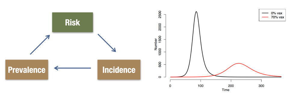
These dependencies create non-linearities over time, as shown in the right panel above. At the beginning of an infectious disease outbreak, there is an exponential growth curve. This may be characterized based on the doubling time in cumulative case counts. Epidemic potential can also be quantified with R0, which average number of transmissions resulting an infected individual in a completely susceptible population. The 0 in R0 refers to the time 0 in an epidemic when this would be the case; colloquially, people also use R0 to discuss epidemic potential at later time points. Therefore, R0 might shrink over time as the susceptible population is depleted, or as different behavioral or biological interventions are implemented.
Mathematical models for epidemics take parameters like R0 as inputs. Models then construct the mechanisms to get from the micro-level (individual-level biology, behavior, and demography) to the macro-level (population disease incidence and prevalence). This construction depends heavily on theory, often supported by multiple fields of empirical science that provides insight into how the mechanisms (gears in the diagram below) fit together individually and together in the system.
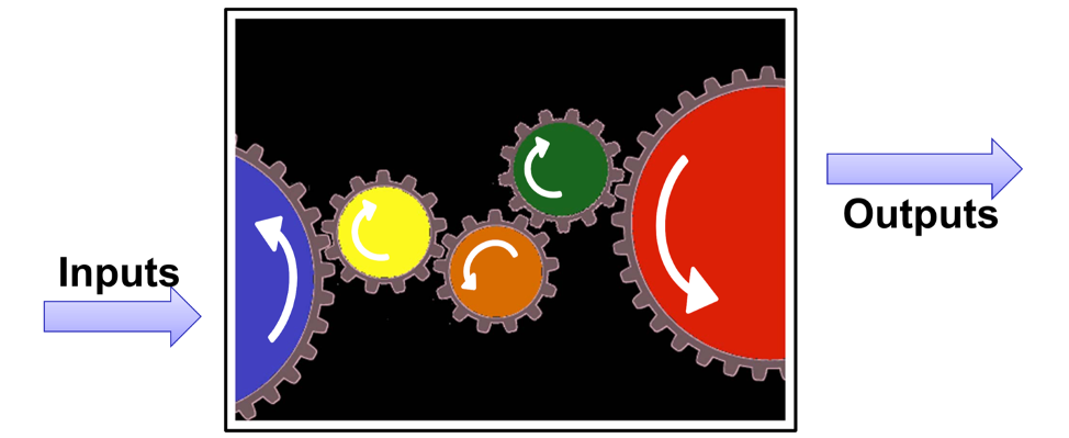
Because of the complexity of these systems, and the wide range of mechanisms embedded, models typically synthesize multiple data streams from interdisciplinary scientific fields. Flexibility with data inputs is also important during disease outbreaks, when the availability of large cohort studies or clinical trials to explain the disease etiology or interventions with precision may be limited.
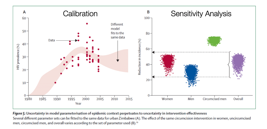
Fortunately, there are several statistical methods for evaluating the consistency of the hypothesized model against nature. Model calibration methods that test what model parameter values (e.g., values of R0) are more or less consistent with data (e.g., case surveillance of diagnosed cases). Sensitivity analyses quantify how much the final projections of a model (e.g., the effect of an infectious disease intervention) depend on the starting model inputs.
Putting these pieces together, models provide a virtual laboratory to test different hypotheses about the often complex and counterintuitive relationships between inputs and outputs. This virtual laboratory not only allows for estimation of projected future outcomes, but also testing of counterfactual scenarios for which complete data may not be available.
How Are Models Built and Analyzed?
There are many classes of mathematical models used within epidemiology. Three broad categories are: deterministic compartmental models (DCMs), agent-based models (ABMs), and network models. DCMs divide the population into groups defined, at a minimum, by the possible disease states that one could be in over time. ABMs and network models represent and simulate individuals rather than groups, and they provide a number of advantages in representing the contact processes that generate disease exposures. DCMs are the foundation of mathematical epidemiology, and provide a straightforward introduction to how models are built.
Take the example in the figure below of an immunizing disease like influenza or measles, which can be characterized by the disease states of susceptible (compartment S), infected (compartment I), and recovered (compartment R). Persons start out in S at birth, then move to I, and then to R. The flow diagram, kind of like a DAG, defines the types of transition that are hypothesized to be possible (and by an omission of arrows, which are hypothesized not). Movement from S to I corresponds to disease transmission, and the movement from I to R corresponds to recovery. There may be additional exogenous in-flows and out-flows, like those shown in the diagram, that correspond to births and deaths.
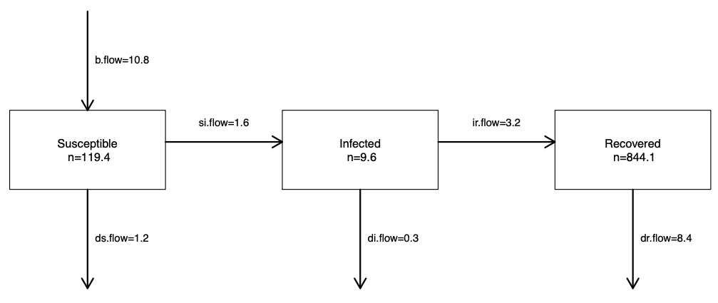
The speed at which transmission and recovery occur over time is controlled by model parameters. These flow diagrams are translated into mathematical equations that formally define this model structure and the model parameters. The following set of equations that correspond to this figure. These are differential equations that specify, on the left-hand side, how fast the sizes of the compartments change (the numerators) over time (the denominator). On the right-hand side are the definition of the set of flows in and out of each compartment.
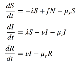
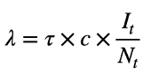
One flow, from the S to I compartment, includes the λ (lambda) parameter that defines the “force of infection.” This is the time-varying rate of disease transmission. It varies over time for the reasons shown in the epidemic feedback loop diagram, shown above, and formalized in the equation below. The rate of disease transmission per unit of time can be defined as the rate of contact per time, c, times the probability that each contact will lead to a transmission event, t, times the probability that any contact is with an infected person. The last term is another way of expressing the disease prevalence; this is the feature of the feedback loop that changes over time as the epidemic plays out.
The overall size of transitions is therefore a function of these model parameters and the total size of the compartments that the parameters apply to. In the case of disease transmission, the parameters apply to people who could become infected, or people in the S compartment. Once all the equations are built, they are programmed in a computer, such as the software tool for modeling that I built called EpiModel. To experiment with a simple DCM model, check out our Shiny app.
More complex models build out the possible disease states, for example, by adding a latently infected but un-infectious stage (called SEIR models). Or they add another transition, by adding an arrow from R back to S in the case that immunity is temporary (called SIRS models). Or they add extra stratifications, such as age groups, when those strata are relevant to the disease transmission or recovery process. By adding these stratifications, different assumptions about the contact process are then possible; for example, by simulating a higher contact rate for younger persons or concentrating most of the contacts of young people with other young people. These additional model structures should be based on good theory, supported by empirical data.
How Have Models Been Used to Understand COVID-19?
Mathematical models have been used broadly in two ways in the current COVID-19 global pandemic: 1) understanding what has just happened to the world or what will soon happen; 2) figuring what to do about it.
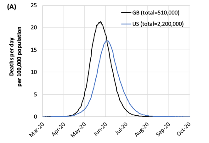
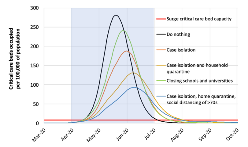
In the first category, several models have estimated the burden of disease (cases, hospitalizations, deaths) against healthcare capacity. The most famous of these models is the “Imperial College” model, led by investigators at that institution, and published online on March 16. This is an agent-based model that first projected the numbers of deaths and hospitalizations of COVID in the U.K. and the U.S. against current critical care capacity under different scenarios. In the “do nothing” scenario, in which there were no changes to behavior, the model projected 2.2 million deaths would occur in the U.S. and over 500,000 in the U.K.
The model also included scenarios of large-scale behavioral change (an example of the second category of use, what to do about it), in which different case isolation and “social distancing” (a new addition to the lexicon) measures were imposed. Under these scenarios, we could potentially “flatten the curve,” which meant reducing the peak incidence of disease relative to the healthcare system capacity. These changes were implemented in the model by changing the model parameters related to the contact rates; in this case, the model structure and the contact rates were stratified by location of contacts (home, workplace, school, community) and age group.
After these models were released, the U.S. federal government substantially changed its recommendations related to social distancing nationally. There was subsequent discussion about how long these distancing measures needed to be implemented, because of the huge social and economic disruption that these changes entailed. One high-stakes policy question was whether these changes could be relaxed by Easter in mid-April or perhaps early Summer.
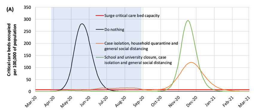
The Imperial College model suggests that as soon as the social distancing measures are relaxed (in the purple band) there will be a resurgence of new cases. This second wave of infection was driven by the fact that the outbreak would continue in the absence of any clinical therapy to either prevent the acquisition of disease (e.g., a vaccine) or reduce its severity (e.g., a therapeutic treatment). Particularly concerning with these incremental distancing policies would be if the second wave occurred during the winter months later this year, which would coincide with seasonal influenza.
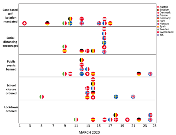
An update to the Imperial College model was released on March 30. This model projected a much lower death toll in the U.K. (around 20,000 cases, compared to over 500,000 in the earlier model). This was interpreted by some news reports as an error in the earlier model. But instead, this revised model incorporated the massive social changes that were implemented in the U.K. and other European countries over the month of March, as shown in the figure below. Adherence to these policies were estimated to have prevented nearly 60,000 deaths during March.
This is just one of many mathematical models for COVID. Several other examples of interest are included in the resource list below. There has been an explosion of modeling research on COVID since the initial outbreak in Wuhan, China in early January. This has been facilitated by the easy sharing of pre-print papers, along with the relatively low threshold in building simple epidemic models. With this explosion of research, much of the world has become interested with modeling research as the model projections are very relevant to daily life, and fill the gap in the news coverage in advance with clinical advances in testing, treatment, and vaccine technologies. Because pre-prints have not been formally vetted in peer review, it can be challenging for non-modelers (including news reporters and public health policymakers) to evaluate the quality of modeling projections. We have seen several cases already where nuanced modeling findings have been misinterpreted or overinterpreted in the news.
As the adage by George Box goes: all models are wrong, but some are useful. This applies to mathematical models for epidemics too, including those for COVID-19. Useful models are informed by good data, and this data collection usually takes time. These data inputs for models may rapidly change as well, as was the case for the updated Imperial college model, so earlier model projections may be outdated. This does not mean that the earlier model was wrong. In one sense, models prove their utility in the absence of bad news if they stimulate public action towards prevention, which may have an effect on the shape of the future epidemic curve. In the short-term, public consumers of models may not be able to fully determine the technical quality of that research. But it is important to understand that priorities of newspapers and politicians, and what they find useful in some models, may differ substantially from strong scientific principles.
Resources
There are many resources for learning more about modeling, including my Spring Semester course at RSPH, EPI 570 (Infectious Disease Dynamics: Theory and Models). We use the textbook, An Introduction to Infectious Disease Modeling, by Emilia Vynnycky & Richard White, that provides an excellent overview of modeling basics. We also have open materials available for our summer workshop, Network Modeling for Epidemics, that focuses specifically on stochastic network models.
In addition, here is a short list of interesting and well-done COVID modeling studies:
- Original Imperial College model: https://www.imperial.ac.uk/media/imperial-college/medicine/sph/ide/gida-fellowships/Imperial-College-COVID19-NPI-modelling-16-03-2020.pdf
- Updated Imperial College model: https://www.imperial.ac.uk/media/imperial-college/medicine/mrc-gida/2020-03-30-COVID19-Report-13.pdf
- Model of social distancing in Wuhan: https://www.thelancet.com/journals/lanpub/article/PIIS2468-2667(20)30073-6/fulltext
- Social distancing model for repeated episodic distancing measures: https://dash.harvard.edu/handle/1/42638988
- Interactive model on the NY Times: https://www.nytimes.com/interactive/2020/03/25/opinion/coronavirus-trump-reopen-america.html
- Age profile of the COVID epidemic: https://dash.harvard.edu/handle/1/42639493
- Model of outbreak on the Diamond Princess cruise ship: https://academic.oup.com/jtm/advance-article/doi/10.1093/jtm/taaa030/5766334

Samuel Jenness, PhD is an Assistant Professor in the Department of Epidemiology at the Rollins School of Public Health at Emory University. He is the Principal Investigator of the EpiModel Research Lab, where the research focuses on developing methods and software tools for modeling infectious diseases. Our primary applications are focused on understanding HIV and STI transmission in the United States and globally, as well as the intersection between infectious disease epidemiology and network science.