Rubicon Rehabilitation Center in the Virginia Press 1971-1976

Rubicon Rehabilitation Center in the Virginia Press 1971-1976

Rubicon Graduates Celebrating: Photo from Rubicon Current vol 2. Box 60 Folder 15, The Papers of Stanley Clay Walker, Special Collections and University Archives, Patricia W. and J. Douglas Perry Library, Old Dominion University Libraries, Norfolk, VA.


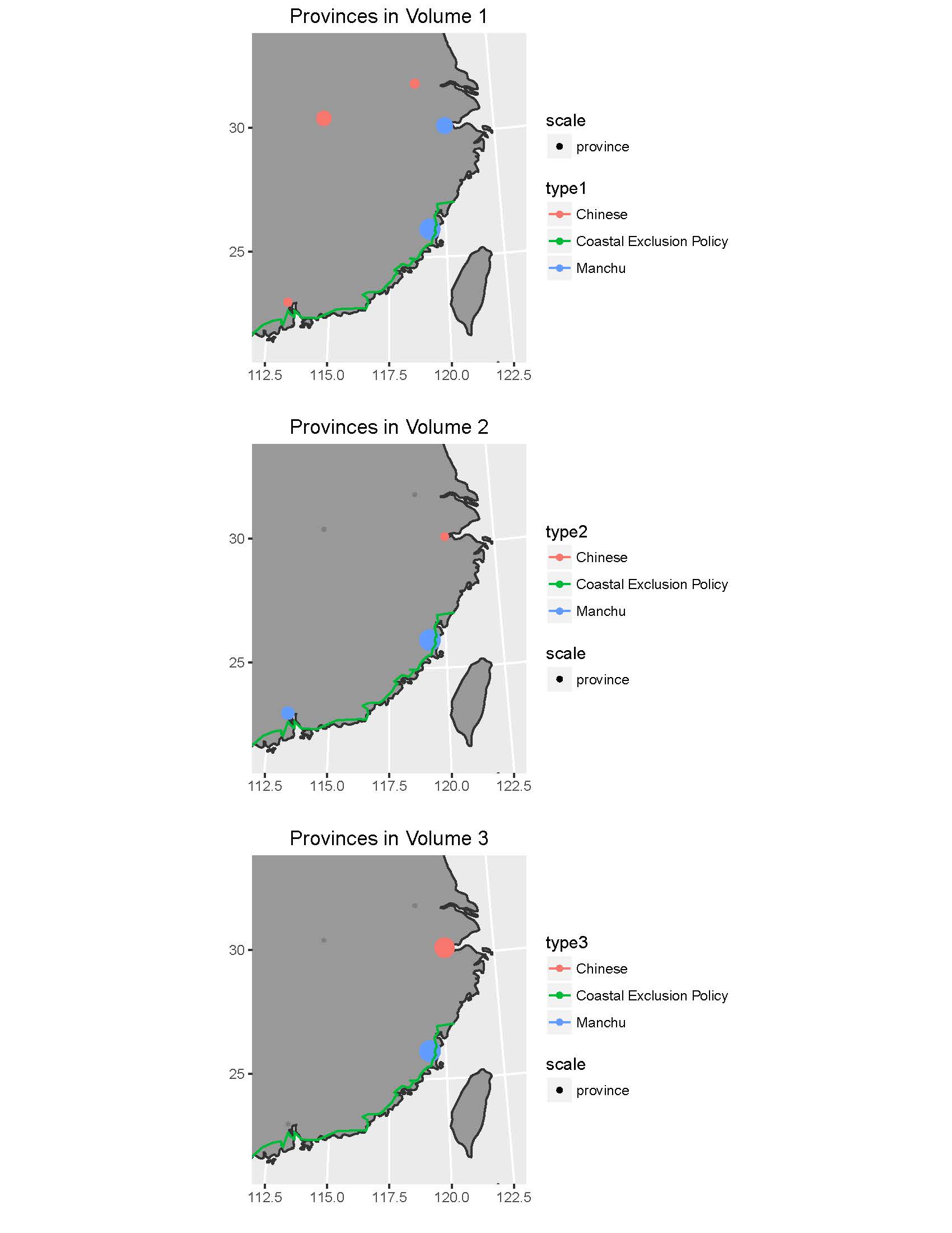
By 1971 Rubicon had become the largest in-patient rehabilitation program in the state of Virginia, maintaining extensive partnerships with the Department of Vocational Rehabilitation, the Medical College of Virginia(MCV), Richmond City Health Department, and the Richmond Public School system. Through its partnership with MCV it became the only federally approved methadone program between Washington D.C. and Miami.1   In a time where the merits and demerits of drug abuse treatment were in constant debate internationally Rubicon became the medium through which newspapers throughout the state of Virginia localized rehabilitation issues. By using the text-mining tools in R and a corpus of 80 newspapers from five different cities in Virginia a glimpse of this conversation can be gained.

The Corpus Over Time


The Danville Register, The Harrisonburg Daily Record, The Norfolk Journal and Guide, The Petersburg Progress Index, The Winchester Star

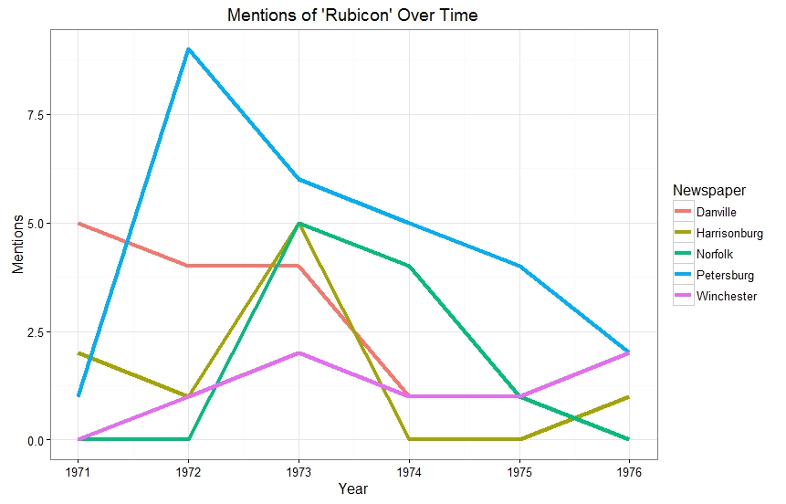
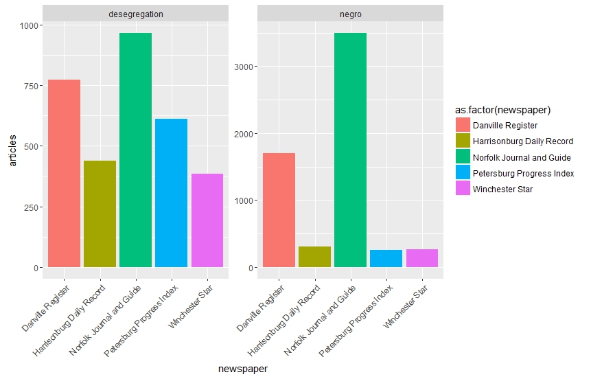
The graph above shows that mentions of Rubicon generally declined over time. This is probably dues to several factor: the decline in novelty, the slowing of intake at Rubicon, and shifting drug control priorities. It also reveals the relationship Rubicon had with Petersburg. Many of Rubicon’s admits were funneled to them through the Petersburg court system. Interestingly enough mentions in the two cities with the Rubicon facilities near there localities drop of in 1973. This is in line with larger statewide drug arrest trends that show a dip in arrests in 1973.

Most Characteristic Words in the Corpus

tf-idf-formula


Using TF-IDF(term frequency-inverse document frequency) statistic to extract key terms from the four newspapers that wrote the most about Rubicon can provide a distant look at the semantic difference between newspapers. For more on TF-IDF see Kan Nashida’s blog.


tfidf


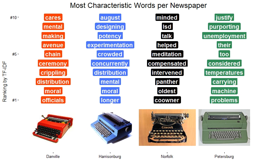
As can be seen TF-IDF produces some interesting results. The Danville newspaper uses words like “cares, “ceremony”, and “morals”, showing an interest in the positive impact of Rubicon. It also uses words like “chain”,”officials”, and “mental” which may reflect an interest in the organizational mechanics of Rubicon.  Similarly, Harrisonburg uses words like  “experimentation”, “crowded”, and, “designing” that imply and interest in how Rubicon was ran and maintained. The overlap of words between Harrisonburg and Danville may be due to proximity. The two cities were farther away from Rubicon then Norfolk and Petersburg and likely relied on the same AP reports. The Norfolk Journal and Guide is the only historically black newspaper in the corpus and discusses the black panthers more according to the TF-IDF metric. It is also the only newspaper that has a drug word(LSD) in its top ten of most characteristic words. Words like “mediated”, “helped”, and, “intervened” point to the expansion of Rubicon into the Norfolk area in 1973. Words in the Petersburg Progress Index reflect a similar closeness between Petersburg and Rubicon. “Unemployment”, “problems” and the disproportionately frequent use of “their” signify close economic and organizational ties.

Correlations

Correlation Matrices are another text-mining tool that can help shed light on Rubicon without a close reading. Correlations measure the strength of the relationship between variables. A correlation <0 indicates a negative relationship while a correlation>0 indicates a positive relationship.

rubicon-dem-corr


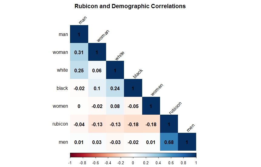
The matrix above shows a close correlation between the word “Rubicon” and the plural “men” across the whole corpus. On the other hand, it also shows a negative correlation between “Rubicon”, and the plural “women”. Surprisingly, race did not play a significant role in the coverage of Rubicon in the newspapers even though it appeared frequently throughout the press during this period.

race

rubicon-and-justice


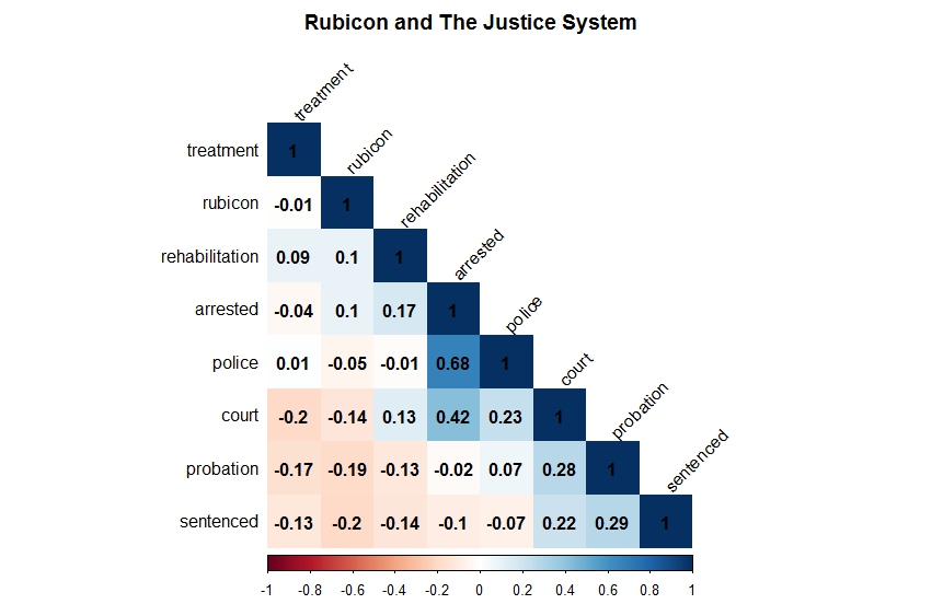
Rubicon’s relationship with the workings of the justice system is a bit more nuanced. Its important to remember that all of the newspapers mention Rubicon. The fact that Rubicon does not correlate highly with “rehabilitation” and “treatment” shows that Rubicon had reached a level of public notoriety that it no longer had to be described using these terms. Even so there is still a positive correlation between it and the words “arrested” and “court.”

kelly-and-menken


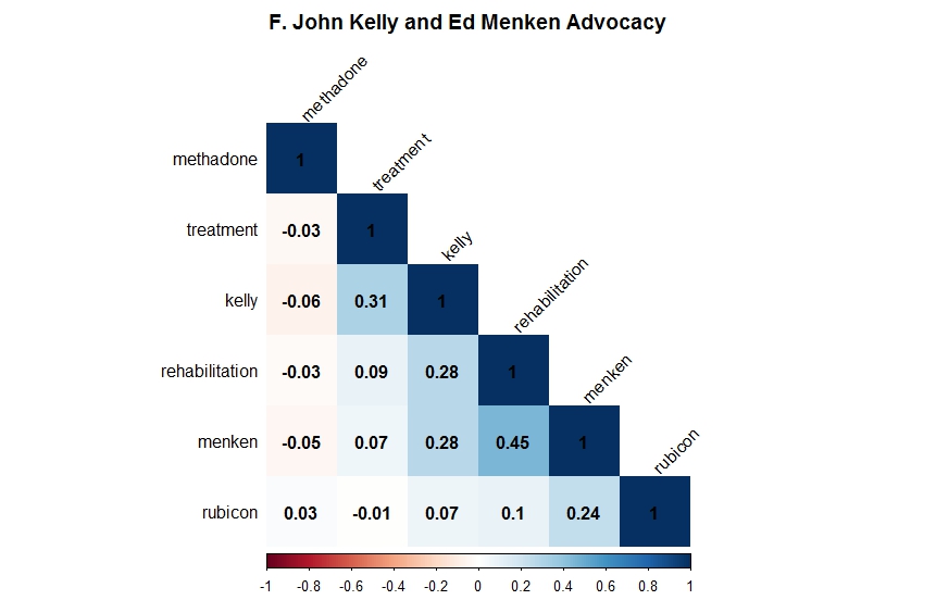
F. John Kelly, the director of the Governor’s Council on Narcotics and Drug Abuse Control, and Ed Menken the director of Rubicon had a sometimes contentious relationship in the press.  Menken frequently accused Kelly of taking a soft approach toward drug rehabilitation. The graphic above shows that Kelly correlates more highly with “treatment” but not “rehabilitation” than Menken. This could just be a matter of different word choices between the two after all Kelly is mentioned in 12 different articles while Menken is only mentioned in 6.

The positive correlation between Kelly and Menken denotes the level of dialog between the two. From the view of the frequent newspaper reader Kelly and Menken were locked in constant debate over rehabilitation resources and agendas. This constant pairing would have made Menken seem less like the Director of a private rehab and more like Kelly political equivalent. Another surprise from figure 6 is the lack of correlation between Kelly, Menken, and Rubicon with the word “methadone.”  Despite their advocacy for rehabilitation and treatment neither Kelly or Menken wanted to broach the controversial topic of methadone.

 Conclusion


correlation


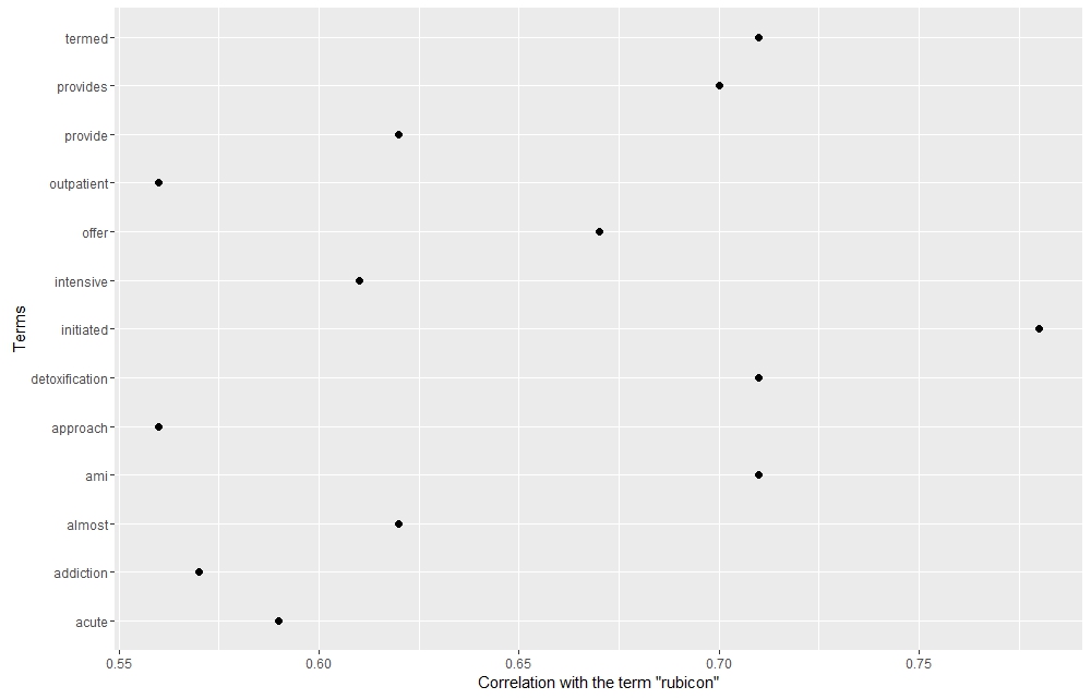
By analyzing the terms that correlate with Rubicon its institutional identity clearly exceeds that of its grassroots activist identity. Clinical terms like “detoxification”, “termed”, “outpatient”, “intensive”, “acute”, “provide”, and “offer” speak the business and medical side of the organization, and perhaps signify its movement toward a rehab ran by medical professionals rather than former addicts.  Coverage of Rubicon in the Virginia press neutralized the racial and activist components of the organization, thus helping to perpetuate the image of it as a state institution that both engaged in policy discussions and became a component of the justice system.

Code

library(stringr)
 library(corrplot)
 library(ggplot2)
 Convert Download articles into .txt and place in dataframe
 # folder with article PDFs
 dest <- "C:\\Users\\virgo\\Desktop\\Rubicon"
 # make a vector of PDF file names
 myfiles # convert each PDF file that is named in the vector into a text file
 # text file is created in the same directory as the PDFs
 # use pdftotxt.exe
 lapply(myfiles, function(i) system(paste('"C:\\Users\\Virgo\\Destop\\xpdf/bin64/pdftotext.exe"', paste0('"', i, '"')), wait = FALSE) )
 #create vector of txt file names
 rubiconfiles<-list.files(path = dest, pattern= "txt", full.names = TRUE)
 #turn into a list
 obj_list rubicon<-data.frame(obj_list)
 Clean up rubicon
 ##import rubicon.csv
 ##convert article text into lowercase and turn it into a string
 rubicon$Text<-tolower(rubicon$Text)
 rubicon.string ## split the string into words
 rubicon.string Word.list.df colnames(Word.list.df) ## remove blanks,lower, numbers
 Word.list.df Word.list.df$word<-tolower(Word.list.df[,1])
 Word.list.df ###create DTM
 target.list DTM.df ncol = length(target.list)))
 for (i in seq_along(target.list))
 {
 DTM.df[,i] }
 colnames(DTM.df) #nornalize DTM
 total.words DTM.matrix DTM.matrix DTM.norm.df #For Figure 2
 ###import rubicon mentions.csv and create line graph that shows mention of rubicon overtime
 ggplot(yy, aes(Year,Mentions))+geom_line(aes(colour=Newspaper), size=1.5)+labs(title="Mentions of 'Rubicon' Over Time") + xlab("Year") + ylab("Mentions") +theme_bw()
 For Correlations
 ##correlation
 short.list DTM.norm.mini.df #To get the correlation matrix
 cor.matrix.mini round(cor.matrix.mini, 2) ## rounds off at 2 places
 corrplot(cor.matrix.mini, method="shade",shade.col=NA,tl.col="black",tl.srt=45,addCoef.col="black",order="AOE", type="lower",title="Rubicon and Demographic Correlations",mar=c(0,0,2,0) )
 For Figure 8
 #word associations
 findAssocs(DTM, "rubicon", 0.57)
 #build dataframe for plotting
 toi <- "rubicon" # term of interest
 corlimit rubiconterms Terms = names(findAssocs(DTM, toi, corlimit)[[1]]))
 ggplot(rubiconterms, aes( y = Terms)) +geom_point(aes(x = corr), data = rubiconterms, size=2) +xlab(paste0("Correlation with the term ", "\"", toi, "\""))
 For Figure 3
 library(tm)
 library(RWeka)
 library(stringr)
 #import rubicon.csv and condense into articles by paper
 by.paper<-NULL
 for(paper in unique(rubicon$X4)){
 subset text row by.paper }
 # create corpus
 myReader corpus # pre-process text
 corpus corpus corpus corpus corpus # create term document matrix
 tdm<-TermDocumentMatrix(corpus)
 # remove sparse terms
 tdm. # save as a simple data frame
 count.all count.all$word write.csv(count.all, "C:\\Users\\virgo\\Desktop\\folder\\tdm.csv", row.names=FALSE)
 #normalize
 ## paste the text into one long string
 big.string ## split the string into words
 big.string ## get a dataframe of word frequency
 Word.list.df ## give the dataframe some nice names
 colnames(Word.list.df) ## remove blanks
 Word.list.df ## add \\b so the words are ready for regex searches
 target.list Word.list.df function(x) str_count(by.paper$text, x)
 count.matrix <-
 sapply(X = target.list, FUN = function(x) str_count(by.paper$text, x))
 ## lines below are clean up
 DTM.df colnames(DTM.df) DTM.matrix DTM.matrix DTM.norm.df paper.tfidf.df function(x) x*log(nrow(DTM.norm.df)/(sum(x!=0)+1))))
 rownames(paper.tfidf.df)<-c("Danville","Harrisonburg","Petersburg","Radford","Winchester","Norfolk")
 x<-6
 Tfidf.ten.df ## transpose for easier sorting
 Tfidf.ten.df ## add words
 Tfidf.ten.df$words ## sort and get top ten
 tfidf.ten tfidf.ten$words
 ###plot tfidf
 n p d h mycolors colnames(p)[1]<-"paper"
 colnames(p)[2]<-"word"
 ggplot(p, aes(paper, rank)) +
 geom_point(color="white") +
 geom_label(aes(label=p$word,fill=p$paper), color='white', fontface='bold', size=5) +
 scale_fill_manual(values = mycolors) +
 theme_classic() +
 theme(legend.position=1,plot.title = element_text(size=18), axis.title.y=element_text(margin=margin(0,10,0,0))) +
 labs(title="Most Characteristic Words per Newspaper") +
 xlab("") + ylab("Ranking by TF-IDF") +
 scale_y_continuous(limits=c(-4,10), breaks=c(1,6,10), labels=c("#1","#5", "#10")) +
 annotation_custom(Norfolk, xmin=.5, xmax=1.5, ymin=0, ymax=-4) +
 annotation_custom(Petersburg, xmin=1.5, xmax=2.5, ymin=0, ymax=-4) +
 annotation_custom(Danville, xmin=2.5, xmax=3.5, ymin=0, ymax=-4) +
 annotation_custom(Harrisonburg, xmin=3.5, xmax=4.5, ymin=0, ymax=-4)
 For Figure 5
 #import csv or race articles numbers
 p<-ggplot(race,aes(x=newspaper, y=articles,fill=as.factor(newspaper))) + geom_bar(stat="identity")+facet_wrap(~word, scales = "free")+theme(axis.text.x = element_text(angle = 45, hjust = 1))


The statistic results on map

The difference of percentage (provinces scale) between Manchu and Chinese version on map combines the line of the Coastal Exclusion Policy.
rplot04

The difference of percentage (cities scale) between Manchu and Chinese version on map combines the line of the Coastal Exclusion Policy.

rplot05

Coding is below.

##————————————————————————————————–##

rm(list=ls())
fileEncoding= “UTF-8”

## read file
setwd(“~/Desktop/003_PhD/016_Coursework/003_2016 Fall/003_HIST582A/003_Text”)
library(stringr)

## scan Chinese and Manchu texts
Chinese.vol.1.txt <- scan(“PDHF_Chinese_1.txt”, what = “chr”)
Chinese.vol.2.txt <- scan(“PDHF_Chinese_2.txt”, what = “chr”)
Chinese.vol.3.txt <- scan(“PDHF_Chinese_3.txt”, what = “chr”)
Manchu.vol.1.txt <- scan(“PDHF_Manchu_1.txt”, what = “chr”)
Manchu.vol.2.txt <- scan(“PDHF_Manchu_2.txt”, what = “chr”)
Manchu.vol.3.txt <- scan(“PDHF_Manchu_3.txt”, what = “chr”)

##————————————————————————————————–##
## [toponym counts] ##
## read table of place names in Chinese, Manchu, and English
Ch.place.names <- read.table(“Chinese_place_names.txt”, stringsAsFactors = FALSE)
Man.place.names <- read.table(“Manchu_place_names.txt”, sep=”\t”, stringsAsFactors = FALSE)
Eng.place.names <- read.table(“English_place_names.txt”, sep=”\t”, stringsAsFactors = FALSE)

## creating a new colname
Man.place.names$places <- tolower(Man.place.names$V1)
Ch.place.names$places <- tolower(Ch.place.names$V1)
Eng.place.names$places <- tolower(Eng.place.names$V1)
Ch.toponym <- unique(Ch.place.names$V1)
Man.toponym <- unique(Man.place.names$places)
Eng.toponym <- unique(Eng.place.names$V1)

## paste the full text
Manchu1 <- tolower(paste(Manchu.vol.1.txt, collapse = ” “))
Manchu2 <- tolower(paste(Manchu.vol.2.txt, collapse = ” “))
Manchu3 <- tolower(paste(Manchu.vol.3.txt, collapse = ” “))
Chinese1 <- paste(Chinese.vol.1.txt, collapse = “”)
Chinese2 <- paste(Chinese.vol.2.txt, collapse = “”)
Chinese3 <- paste(Chinese.vol.3.txt, collapse = “”)

## make the full Chinese text as a dataframe
Ch.Texts.df <- rbind.data.frame(Chinese1, Chinese2, Chinese3, stringsAsFactors = FALSE)
Chinese_all <- paste(Ch.Texts.df, collapse =””)
Ch.Texts.df <- rbind.data.frame(Chinese1, Chinese2, Chinese3, Chinese_all, stringsAsFactors = FALSE)

## rename the colname
colnames(Ch.Texts.df) <- “texts”

Ch.Text.metrics <- data.frame(t(data.frame(lapply(Ch.toponym, FUN=function(x) str_count(Ch.Texts.df$texts, x)))))

## put the place as one colname
Ch.Text.metrics$places <- Ch.toponym

## make three colnames sequently
colnames(Ch.Text.metrics)[c(1:4)] <- c(“Chinese1”, “Chinese2”, “Chinese3”, “Chinese_all”)

## the same process of Chinese in the Manchu version
Man.Texts.df <- rbind.data.frame(Manchu1, Manchu2, Manchu3, stringsAsFactors = FALSE)
Manchu_all <- tolower(paste(Man.Texts.df, collapse = ” “))
Man.Texts.df <- rbind.data.frame(Manchu1, Manchu2, Manchu3, Manchu_all, stringsAsFactors = FALSE)
colnames(Man.Texts.df) <- “texts”

Man.Text.metrics <- data.frame(t(data.frame(lapply(Man.toponym, FUN=function(x) str_count(Man.Texts.df$texts, x)))))

Man.Text.metrics$places <- Man.toponym
colnames(Man.Text.metrics)[c(1:4)] <- c(“Manchu1”, “Manchu2”, “Manchu3”, “Manchu_all”)

## combine Chinese and Manchu dataframe together
Combined.df <- cbind.data.frame(Ch.Text.metrics, Man.Text.metrics)
Combined.df$Chinese1.perc <- Combined.df$Chinese1/sum(Combined.df$Chinese1)*100
Combined.df$Chinese2.perc <- Combined.df$Chinese2/sum(Combined.df$Chinese2)*100
Combined.df$Chinese3.perc <- Combined.df$Chinese3/sum(Combined.df$Chinese3)*100
Combined.df$Chinese_all.perc <- Combined.df$Chinese_all/sum(Combined.df$Chinese_all)*100
Combined.df$Manchu1.perc <- Combined.df$Manchu1/sum(Combined.df$Manchu1)*100
Combined.df$Manchu2.perc <- Combined.df$Manchu2/sum(Combined.df$Manchu2)*100
Combined.df$Manchu3.perc <- Combined.df$Manchu3/sum(Combined.df$Manchu3)*100
Combined.df$Manchu_all.perc<- Combined.df$Manchu_all/sum(Combined.df$Manchu_all)*100

## show the result
Combined.df$toponym <- paste(Combined.df[,10], Combined.df[,5], Eng.place.names$places, sep=” “)
Combined.df$toponym

##————————————————————————————————–##
## [Coastal exclusion policy] ##
library(ggmap)
chinastate.map<-get_map(location=”china”, zoom=10, maptype=”satellite”)

cities.cep<- c(“廣西壯族自治區欽州市”, “廣西壯族自治區北海市合浦縣”, “合浦县石城村”, “廣東省湛江市遂溪县乾留”,
“湛江市雷州市海康港”, “湛江市雷州市扶茂”, “廣東省湛江市徐聞縣”, “廣東省湛江市徐聞縣海安鎮”,
“廣東省湛江市雷州市深田村”, “廣東省湛江市雷州市”, “廣東省湛江市遂溪縣”, “廣東省湛江市遂溪縣長坡墩”,
“廣東省湛江市吴川市博茂”, “廣東省湛江市吳川市”, “廣東省茂名市電白區”,
“廣東省陽江市陽西縣雙魚村”, “廣東省陽江市”, “江門市恩平市”, “廣東省江門市開平市”, “新會區將軍山旅遊區”,
“廣東省江門市新會區崖門鎮”, “廣東省江門市新會區”, “新會區觀音山”, “佛山市順德區”, “中山市三角鎮”,
“中山市馬鞍村”, “南沙区小虎山”, “深圳市寶安區西鄉”, “深圳市大鵬所城”, “海丰县琵琶”, “廣東省汕尾市海豐縣”,
“揭陽市惠來縣”, “揭陽市惠來縣靖海鎮”, “广东省汕头市潮南区古埕”, “廣東省汕頭市潮陽區”,
“揭陽市揭東區鄒堂”, “廣東省揭陽市”, “廣東省潮州市”, “潮州市饒平縣”, “福建省漳州市詔安縣分水關”,
“福建省漳州市詔安縣”, “漳州市云霄县油甘公”, “漳州市漳浦縣”, “漳州市漳浦縣橫口圩”, “漳州市龙海市洪礁寨”,
“漳州市龍海市海澄鎮”, “福建省漳州市龍文區江東橋”, “廈門市同安區蓮花村”, “廈門市同安區”, “廈門市翔安區小盈嶺”,
“福建省泉州市南安市大盈”, “福建省晉江”, “福建省泉州市南安市”, “泉州市洛江区洛陽橋”,
“泉州市惠安县石任”, “泉州市泉港区九峰山”, “莆田市荔城區壺公山”, “莆田市涵江區江口鎮”, “福清市高嶺村”,
“福州市福清市”, “長樂市岐陽村”, “馬尾區閩安村”, “福州市連江縣”, “連江縣浦口鎮”, “蕉城區白鶴嶺”,
“福建省寧德市”, “福安市洋尾”, “福安市小留村”, “寧德市福安市”, “福鼎市沙埕鎮”)
geo.cities.cep <- geocode(cities.cep)
geo.cities.cep.df<- data.frame(geo.cities.cep)

ggmap(chinastate.map) + geom_point(data=geo.cities.cep, aes(x=lon, y=lat))+ xlim(c(108, 122)) +ylim(c(20,28))

##————————————————————————————————–##
## [map] ##
library(ggmap)
china.map<-get_map(location=”China”, zoom=10, maptype=”satellite”)

cities<- c(“福建省泉州南安市安平橋”, “福建省廈門市同安區丙洲”, “湖南省長沙市”, “廣東省潮州市”,
“中國福建省泉州市惠安縣崇武鎮”, “中國福建省三明市永安市大漳山”, “福建福州市連江縣定海古城”,
“印尼雅加達”, “福建省寧德市霞浦縣烽火島”, “中國福建省”, “福建省福州市”, “福建省福州市長樂市新塘”,
“江蘇省揚州市邗江區瓜洲鎮”, “中國廣東省”, “中國貴州省”, “福建省漳州市龍海市海澄鎮”,
“福建省福州市平潭縣海壇島”, “福建省福州市台江區河口新村”, “中國湖北省”, “廣東省惠州市”,
“江蘇省南京市”, “廣東省汕尾市陸豐市碣石鎮”, “中國江蘇省”, “金門縣”, “廣東省汕頭市濠江區馬滘”,
“福建省莆田市秀嶼區湄洲大道湄洲島”, “福建省福州市馬尾區閩安村”, “廣東省汕頭市南澳縣”,
“浙江省寧波市”, “普列莫爾斯基區海參崴”, “廣東省汕頭市龍湖區鷗汀”, “臺灣省澎湖”,
“福建省莆田市秀嶼區平海鎮”, “浙江省溫州市平陽縣”, “福建省泉州市”, “浙江省紹興市”,
“福建福州市平潭縣石牌洋”, “福建省泉州石井鎮”, “福建省泉州市惠安縣獺窟島”, “浙江省台州市”,
“臺灣台南”, “福建省龍岩市長汀縣汀州”, “福建省廈門市同安區”, “福建省漳州市東山縣”,
“福建省泉州市惠安縣”, “福建省泉州市晉江市圍頭村”, “浙江省溫州市”, “福建省漳州市龍海市浯嶼”,
“福建省廈門市翔安區斗門”, “福建省廈門市”, “福建省莆田市”, “福建省廈門市集美區潯尾”,
“福建省泉州市石獅市永寧鎮”, “湖南岳陽縣”, “福建省漳州市雲霄縣”, “福建省漳州市”,
“中國浙江省”, “江蘇省鎮江市”, “浙江省舟山市”, “福建省泉州石獅市”)

geo.cities <- geocode(cities)
geo.cities.df<- data.frame(geo.cities)

map.df <- cbind.data.frame(Combined.df, geo.cities.df)

library(maps)
library(mapdata)
library(ggplot2)
world.map<- borders(database=”world”)
ggplot()+ world.map+ coord_quickmap()

world.map<- borders(database=”world”, colour=”gray20″, fill=”gray60″)
ggplot() + world.map +
coord_map(projection = “gilbert”, xlim =c(100,140), ylim=c(-20,50)) +
xlab(“”) + ylab(“”)+ ggtitle(“Percentage difference map”)
##————————————————————————————————–##
## [The new try] ##
## mixed provinces and cities ##
## volume 1 ##
Combined.df$perc1.diff <- (Combined.df$Chinese1.perc – Combined.df$Manchu1.perc)
Combined.df$perc2.diff <- (Combined.df$Chinese2.perc – Combined.df$Manchu2.perc)
Combined.df$perc3.diff <- (Combined.df$Chinese3.perc – Combined.df$Manchu3.perc)
map.df <- cbind.data.frame(Combined.df, geo.cities.df)
map.df$type1 <- ifelse(map.df$perc1.diff>0, “Chinese”, “Manchu”)
map.df$type1 <- ifelse(map.df$perc1.diff == 0, NA, map.df$type1)
map.df$type2 <- ifelse(map.df$perc2.diff>0, “Chinese”, “Manchu”)
map.df$type2 <- ifelse(map.df$perc2.diff == 0, NA, map.df$type2)
map.df$type3 <- ifelse(map.df$perc3.diff>0, “Chinese”, “Manchu”)
map.df$type3 <- ifelse(map.df$perc3.diff == 0, NA, map.df$type3)
map.df$scale <- c(“city”, “city”, “city”, “city”, “city”, “city”, “city”, “province”, “city”,”province”, “city”, “city”, “city”,
“province”, “province”, “city”, “city”, “city”, “province”, “city”, “city”, “city”, “province”, “city”, “city”,
“city”, “city”, “city”, “city”, “city”, “city”, “city”, “city”, “city”, “city”, “city”, “city”, “city”, “city”,
“city”, “city”, “city”, “province”, “city”, “city”, “city”)

## only province in Manchu and Chinese##
## volume 1 ##
vol1bp<- ggplot() + world.map + geom_point(data = subset(map.df, scale== “province”), aes(x = lon, y = lat, color=type1, shape = scale, size=abs(perc1.diff))) +
guides(size = FALSE) +
geom_path(data = geo.cities.cep.df, aes(x = lon, y = lat, color = “Coastal Exclusion Policy”))+
coord_map(projection = “stereographic”, xlim = c(112, 123), ylim = c(21,34)) + ylab(“”) + xlab(“”) +
ggtitle(“Provinces in Volume 1”)

## volume 2 ##
vol2bp<- ggplot() + world.map + geom_point(data = subset(map.df, scale == “province”), aes(x = lon, y = lat, color=type2, shape = scale, size=abs(perc2.diff))) +
guides(size = FALSE) +
geom_path(data = geo.cities.cep.df, aes(x = lon, y = lat, color = “Coastal Exclusion Policy”))+
coord_map(projection = “stereographic”, xlim = c(112, 123), ylim = c(21,34)) + ylab(“”) + xlab(“”) +
ggtitle(“Provinces in Volume 2”)

## volume 3 ##
vol3bp<- ggplot() + world.map + geom_point(data = subset(map.df, scale == “province”), aes(x = lon, y = lat, color=type3, shape = scale, size=abs(perc3.diff))) +
guides(size = FALSE) +
geom_path(data = geo.cities.cep.df, aes(x = lon, y = lat, color = “Coastal Exclusion Policy”))+
coord_map(projection = “stereographic”, xlim = c(112, 123), ylim = c(21,34)) + ylab(“”) + xlab(“”) +
ggtitle(“Provinces in Volume 3”)

##only cities in Manchu and Chinese##
## volume 1##
vol1bc<- ggplot() + world.map + geom_point(data = subset(map.df, scale== “city”), aes(x = lon, y = lat, color=type1, shape = scale, size=abs(perc1.diff))) +
guides(size = FALSE) +
geom_path(data = geo.cities.cep.df, aes(x = lon, y = lat, color = “Coastal Exclusion Policy”))+
coord_map(projection = “stereographic”, xlim = c(112, 123), ylim = c(21,34)) + ylab(“”) + xlab(“”) +
ggtitle(“Cities in Volume 1”)

## volume 2 ##
vol2bc<- ggplot() + world.map + geom_point(data = subset(map.df, scale== “city”), aes(x = lon, y = lat, color=type2, shape = scale, size=abs(perc2.diff))) +
guides(size = FALSE) +
geom_path(data = geo.cities.cep.df, aes(x = lon, y = lat, color = “Coastal Exclusion Policy”))+
coord_map(projection = “stereographic”, xlim = c(112, 123), ylim = c(21,34)) + ylab(“”) + xlab(“”) +
ggtitle(“Cities in Volume 2”)

##volume 3 ##
vol3bc<- ggplot() + world.map + geom_point(data = subset(map.df, scale== “city”), aes(x = lon, y = lat, color=type3, size=abs(perc3.diff))) +
guides(size = FALSE) +
geom_path(data = geo.cities.cep.df, aes(x = lon, y = lat, color = “Coastal Exclusion Policy”))+
coord_map(projection = “stereographic”, xlim = c(112, 123), ylim = c(21,34)) + ylab(“”) + xlab(“”) +
ggtitle(“Cities in Volume 1”)
## this function is from http://kanchengzxdfgcv.blogspot.tw/2016/11/r-ggplot2.html##
multiplot <- function(…, plotlist=NULL, file, cols=1, layout=NULL) {
library(grid)
plots <- c(list(…), plotlist)
numPlots = length(plots)
if (is.null(layout)) {
layout <- matrix(seq(1, cols * ceiling(numPlots/cols)),
ncol = cols, nrow = ceiling(numPlots/cols))
}

if (numPlots==1) {
print(plots[[1]])

} else {
grid.newpage()
pushViewport(viewport(layout = grid.layout(nrow(layout), ncol(layout))))
for (i in 1:numPlots) {
matchidx <- as.data.frame(which(layout == i, arr.ind = TRUE))

print(plots[[i]], vp = viewport(layout.pos.row = matchidx$row,
layout.pos.col = matchidx$col))
}
}
}
## provinces in both##
multiplot(vol1bp, vol2bp, vol3bp, cols= 1)

## cities in both##
multiplot(vol1bc, vol2bc, vol3bc, cols =1)