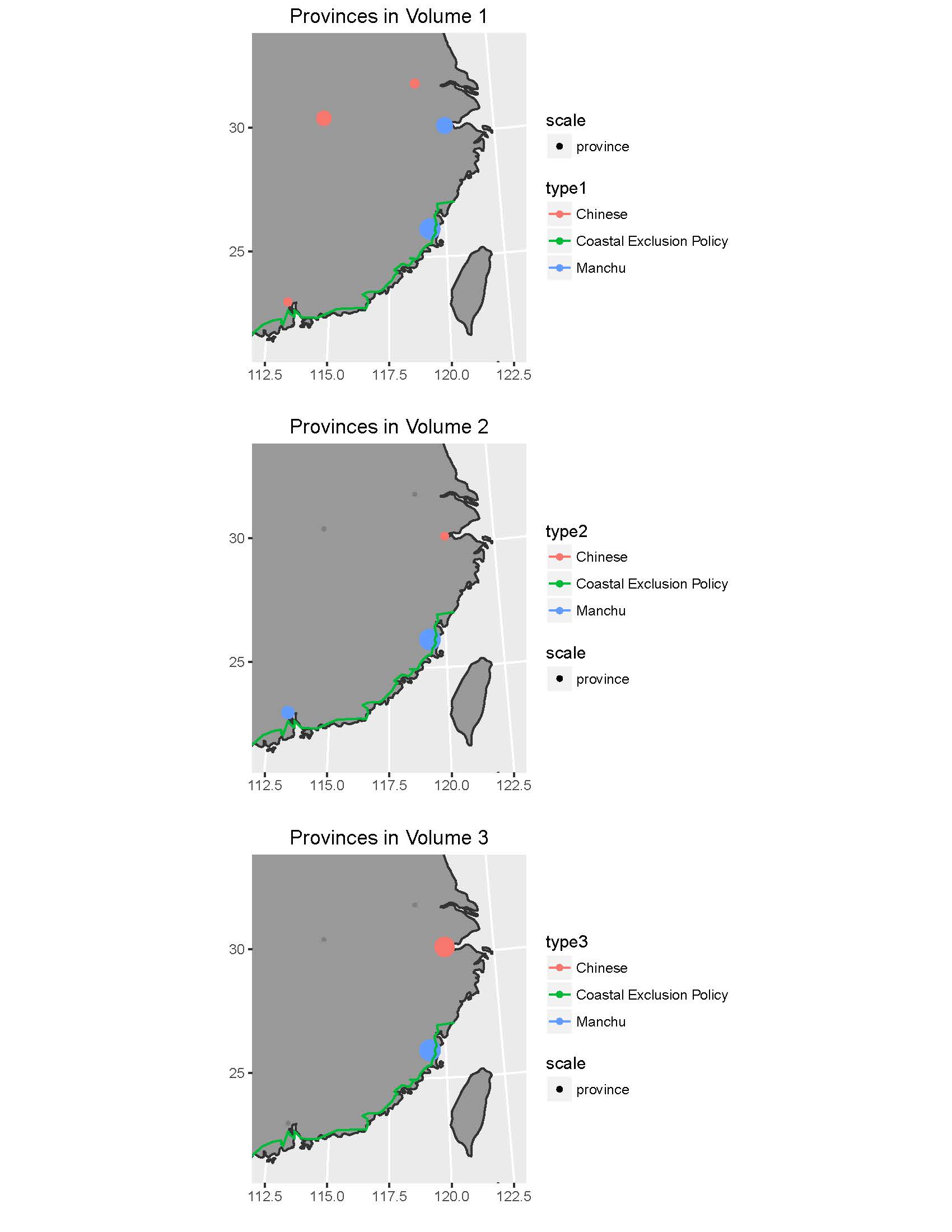
The difference of percentage (provinces scale) between Manchu and Chinese version on map combines the line of the Coastal Exclusion Policy.
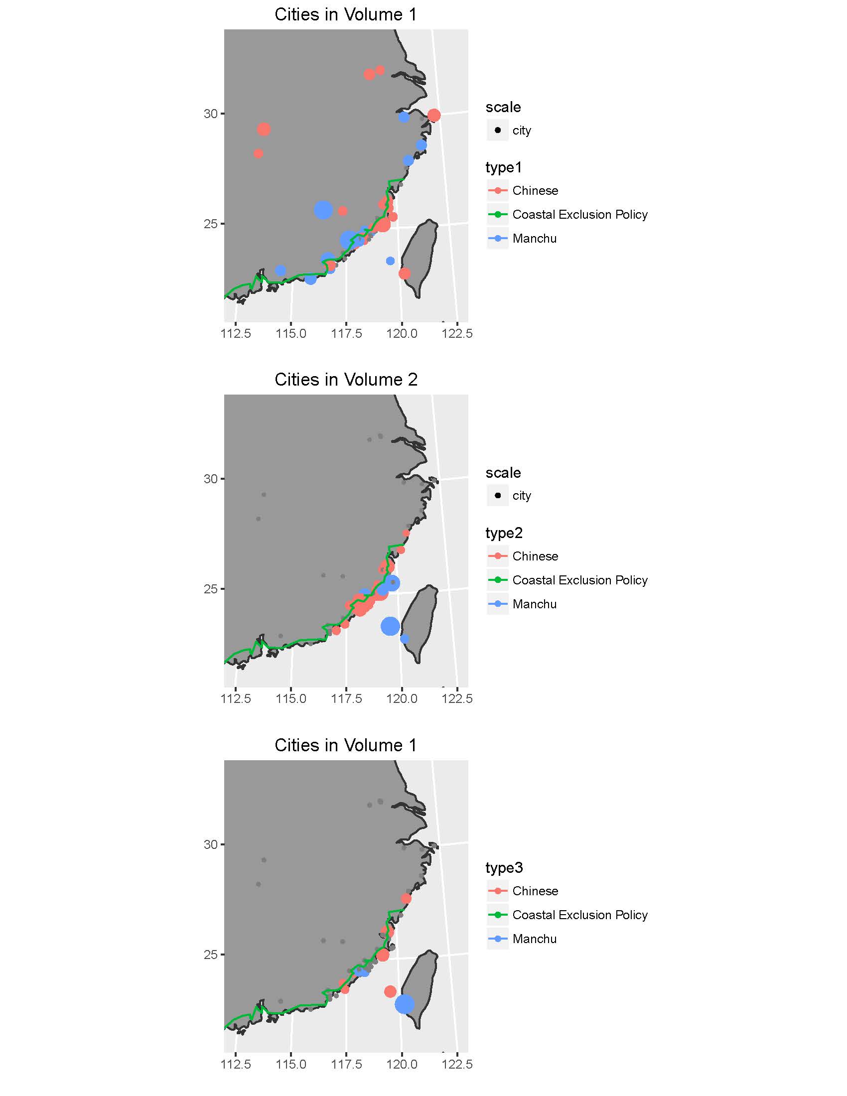
The difference of percentage (cities scale) between Manchu and Chinese version on map combines the line of the Coastal Exclusion Policy.
Coding is below.
##————————————————————————————————–##
rm(list=ls())
fileEncoding= “UTF-8”
## read file
setwd(“~/Desktop/003_PhD/016_Coursework/003_2016 Fall/003_HIST582A/003_Text”)
library(stringr)
## scan Chinese and Manchu texts
Chinese.vol.1.txt <- scan(“PDHF_Chinese_1.txt”, what = “chr”)
Chinese.vol.2.txt <- scan(“PDHF_Chinese_2.txt”, what = “chr”)
Chinese.vol.3.txt <- scan(“PDHF_Chinese_3.txt”, what = “chr”)
Manchu.vol.1.txt <- scan(“PDHF_Manchu_1.txt”, what = “chr”)
Manchu.vol.2.txt <- scan(“PDHF_Manchu_2.txt”, what = “chr”)
Manchu.vol.3.txt <- scan(“PDHF_Manchu_3.txt”, what = “chr”)
##————————————————————————————————–##
## [toponym counts] ##
## read table of place names in Chinese, Manchu, and English
Ch.place.names <- read.table(“Chinese_place_names.txt”, stringsAsFactors = FALSE)
Man.place.names <- read.table(“Manchu_place_names.txt”, sep=”\t”, stringsAsFactors = FALSE)
Eng.place.names <- read.table(“English_place_names.txt”, sep=”\t”, stringsAsFactors = FALSE)
## creating a new colname
Man.place.names$places <- tolower(Man.place.names$V1)
Ch.place.names$places <- tolower(Ch.place.names$V1)
Eng.place.names$places <- tolower(Eng.place.names$V1)
Ch.toponym <- unique(Ch.place.names$V1)
Man.toponym <- unique(Man.place.names$places)
Eng.toponym <- unique(Eng.place.names$V1)
## paste the full text
Manchu1 <- tolower(paste(Manchu.vol.1.txt, collapse = ” “))
Manchu2 <- tolower(paste(Manchu.vol.2.txt, collapse = ” “))
Manchu3 <- tolower(paste(Manchu.vol.3.txt, collapse = ” “))
Chinese1 <- paste(Chinese.vol.1.txt, collapse = “”)
Chinese2 <- paste(Chinese.vol.2.txt, collapse = “”)
Chinese3 <- paste(Chinese.vol.3.txt, collapse = “”)
## make the full Chinese text as a dataframe
Ch.Texts.df <- rbind.data.frame(Chinese1, Chinese2, Chinese3, stringsAsFactors = FALSE)
Chinese_all <- paste(Ch.Texts.df, collapse =””)
Ch.Texts.df <- rbind.data.frame(Chinese1, Chinese2, Chinese3, Chinese_all, stringsAsFactors = FALSE)
## rename the colname
colnames(Ch.Texts.df) <- “texts”
Ch.Text.metrics <- data.frame(t(data.frame(lapply(Ch.toponym, FUN=function(x) str_count(Ch.Texts.df$texts, x)))))
## put the place as one colname
Ch.Text.metrics$places <- Ch.toponym
## make three colnames sequently
colnames(Ch.Text.metrics)[c(1:4)] <- c(“Chinese1”, “Chinese2”, “Chinese3”, “Chinese_all”)
## the same process of Chinese in the Manchu version
Man.Texts.df <- rbind.data.frame(Manchu1, Manchu2, Manchu3, stringsAsFactors = FALSE)
Manchu_all <- tolower(paste(Man.Texts.df, collapse = ” “))
Man.Texts.df <- rbind.data.frame(Manchu1, Manchu2, Manchu3, Manchu_all, stringsAsFactors = FALSE)
colnames(Man.Texts.df) <- “texts”
Man.Text.metrics <- data.frame(t(data.frame(lapply(Man.toponym, FUN=function(x) str_count(Man.Texts.df$texts, x)))))
Man.Text.metrics$places <- Man.toponym
colnames(Man.Text.metrics)[c(1:4)] <- c(“Manchu1”, “Manchu2”, “Manchu3”, “Manchu_all”)
## combine Chinese and Manchu dataframe together
Combined.df <- cbind.data.frame(Ch.Text.metrics, Man.Text.metrics)
Combined.df$Chinese1.perc <- Combined.df$Chinese1/sum(Combined.df$Chinese1)*100
Combined.df$Chinese2.perc <- Combined.df$Chinese2/sum(Combined.df$Chinese2)*100
Combined.df$Chinese3.perc <- Combined.df$Chinese3/sum(Combined.df$Chinese3)*100
Combined.df$Chinese_all.perc <- Combined.df$Chinese_all/sum(Combined.df$Chinese_all)*100
Combined.df$Manchu1.perc <- Combined.df$Manchu1/sum(Combined.df$Manchu1)*100
Combined.df$Manchu2.perc <- Combined.df$Manchu2/sum(Combined.df$Manchu2)*100
Combined.df$Manchu3.perc <- Combined.df$Manchu3/sum(Combined.df$Manchu3)*100
Combined.df$Manchu_all.perc<- Combined.df$Manchu_all/sum(Combined.df$Manchu_all)*100
## show the result
Combined.df$toponym <- paste(Combined.df[,10], Combined.df[,5], Eng.place.names$places, sep=” “)
Combined.df$toponym
##————————————————————————————————–##
## [Coastal exclusion policy] ##
library(ggmap)
chinastate.map<-get_map(location=”china”, zoom=10, maptype=”satellite”)
cities.cep<- c(“廣西壯族自治區欽州市”, “廣西壯族自治區北海市合浦縣”, “合浦县石城村”, “廣東省湛江市遂溪县乾留”,
“湛江市雷州市海康港”, “湛江市雷州市扶茂”, “廣東省湛江市徐聞縣”, “廣東省湛江市徐聞縣海安鎮”,
“廣東省湛江市雷州市深田村”, “廣東省湛江市雷州市”, “廣東省湛江市遂溪縣”, “廣東省湛江市遂溪縣長坡墩”,
“廣東省湛江市吴川市博茂”, “廣東省湛江市吳川市”, “廣東省茂名市電白區”,
“廣東省陽江市陽西縣雙魚村”, “廣東省陽江市”, “江門市恩平市”, “廣東省江門市開平市”, “新會區將軍山旅遊區”,
“廣東省江門市新會區崖門鎮”, “廣東省江門市新會區”, “新會區觀音山”, “佛山市順德區”, “中山市三角鎮”,
“中山市馬鞍村”, “南沙区小虎山”, “深圳市寶安區西鄉”, “深圳市大鵬所城”, “海丰县琵琶”, “廣東省汕尾市海豐縣”,
“揭陽市惠來縣”, “揭陽市惠來縣靖海鎮”, “广东省汕头市潮南区古埕”, “廣東省汕頭市潮陽區”,
“揭陽市揭東區鄒堂”, “廣東省揭陽市”, “廣東省潮州市”, “潮州市饒平縣”, “福建省漳州市詔安縣分水關”,
“福建省漳州市詔安縣”, “漳州市云霄县油甘公”, “漳州市漳浦縣”, “漳州市漳浦縣橫口圩”, “漳州市龙海市洪礁寨”,
“漳州市龍海市海澄鎮”, “福建省漳州市龍文區江東橋”, “廈門市同安區蓮花村”, “廈門市同安區”, “廈門市翔安區小盈嶺”,
“福建省泉州市南安市大盈”, “福建省晉江”, “福建省泉州市南安市”, “泉州市洛江区洛陽橋”,
“泉州市惠安县石任”, “泉州市泉港区九峰山”, “莆田市荔城區壺公山”, “莆田市涵江區江口鎮”, “福清市高嶺村”,
“福州市福清市”, “長樂市岐陽村”, “馬尾區閩安村”, “福州市連江縣”, “連江縣浦口鎮”, “蕉城區白鶴嶺”,
“福建省寧德市”, “福安市洋尾”, “福安市小留村”, “寧德市福安市”, “福鼎市沙埕鎮”)
geo.cities.cep <- geocode(cities.cep)
geo.cities.cep.df<- data.frame(geo.cities.cep)
ggmap(chinastate.map) + geom_point(data=geo.cities.cep, aes(x=lon, y=lat))+ xlim(c(108, 122)) +ylim(c(20,28))
##————————————————————————————————–##
## [map] ##
library(ggmap)
china.map<-get_map(location=”China”, zoom=10, maptype=”satellite”)
cities<- c(“福建省泉州南安市安平橋”, “福建省廈門市同安區丙洲”, “湖南省長沙市”, “廣東省潮州市”,
“中國福建省泉州市惠安縣崇武鎮”, “中國福建省三明市永安市大漳山”, “福建福州市連江縣定海古城”,
“印尼雅加達”, “福建省寧德市霞浦縣烽火島”, “中國福建省”, “福建省福州市”, “福建省福州市長樂市新塘”,
“江蘇省揚州市邗江區瓜洲鎮”, “中國廣東省”, “中國貴州省”, “福建省漳州市龍海市海澄鎮”,
“福建省福州市平潭縣海壇島”, “福建省福州市台江區河口新村”, “中國湖北省”, “廣東省惠州市”,
“江蘇省南京市”, “廣東省汕尾市陸豐市碣石鎮”, “中國江蘇省”, “金門縣”, “廣東省汕頭市濠江區馬滘”,
“福建省莆田市秀嶼區湄洲大道湄洲島”, “福建省福州市馬尾區閩安村”, “廣東省汕頭市南澳縣”,
“浙江省寧波市”, “普列莫爾斯基區海參崴”, “廣東省汕頭市龍湖區鷗汀”, “臺灣省澎湖”,
“福建省莆田市秀嶼區平海鎮”, “浙江省溫州市平陽縣”, “福建省泉州市”, “浙江省紹興市”,
“福建福州市平潭縣石牌洋”, “福建省泉州石井鎮”, “福建省泉州市惠安縣獺窟島”, “浙江省台州市”,
“臺灣台南”, “福建省龍岩市長汀縣汀州”, “福建省廈門市同安區”, “福建省漳州市東山縣”,
“福建省泉州市惠安縣”, “福建省泉州市晉江市圍頭村”, “浙江省溫州市”, “福建省漳州市龍海市浯嶼”,
“福建省廈門市翔安區斗門”, “福建省廈門市”, “福建省莆田市”, “福建省廈門市集美區潯尾”,
“福建省泉州市石獅市永寧鎮”, “湖南岳陽縣”, “福建省漳州市雲霄縣”, “福建省漳州市”,
“中國浙江省”, “江蘇省鎮江市”, “浙江省舟山市”, “福建省泉州石獅市”)
geo.cities <- geocode(cities)
geo.cities.df<- data.frame(geo.cities)
map.df <- cbind.data.frame(Combined.df, geo.cities.df)
library(maps)
library(mapdata)
library(ggplot2)
world.map<- borders(database=”world”)
ggplot()+ world.map+ coord_quickmap()
world.map<- borders(database=”world”, colour=”gray20″, fill=”gray60″)
ggplot() + world.map +
coord_map(projection = “gilbert”, xlim =c(100,140), ylim=c(-20,50)) +
xlab(“”) + ylab(“”)+ ggtitle(“Percentage difference map”)
##————————————————————————————————–##
## [The new try] ##
## mixed provinces and cities ##
## volume 1 ##
Combined.df$perc1.diff <- (Combined.df$Chinese1.perc – Combined.df$Manchu1.perc)
Combined.df$perc2.diff <- (Combined.df$Chinese2.perc – Combined.df$Manchu2.perc)
Combined.df$perc3.diff <- (Combined.df$Chinese3.perc – Combined.df$Manchu3.perc)
map.df <- cbind.data.frame(Combined.df, geo.cities.df)
map.df$type1 <- ifelse(map.df$perc1.diff>0, “Chinese”, “Manchu”)
map.df$type1 <- ifelse(map.df$perc1.diff == 0, NA, map.df$type1)
map.df$type2 <- ifelse(map.df$perc2.diff>0, “Chinese”, “Manchu”)
map.df$type2 <- ifelse(map.df$perc2.diff == 0, NA, map.df$type2)
map.df$type3 <- ifelse(map.df$perc3.diff>0, “Chinese”, “Manchu”)
map.df$type3 <- ifelse(map.df$perc3.diff == 0, NA, map.df$type3)
map.df$scale <- c(“city”, “city”, “city”, “city”, “city”, “city”, “city”, “province”, “city”,”province”, “city”, “city”, “city”,
“province”, “province”, “city”, “city”, “city”, “province”, “city”, “city”, “city”, “province”, “city”, “city”,
“city”, “city”, “city”, “city”, “city”, “city”, “city”, “city”, “city”, “city”, “city”, “city”, “city”, “city”,
“city”, “city”, “city”, “city”, “city”, “city”, “city”, “city”, “city”, “city”, “city”, “city”, “city”, “city”,
“city”, “city”, “city”, “province”, “city”, “city”, “city”)
## only province in Manchu and Chinese##
## volume 1 ##
vol1bp<- ggplot() + world.map + geom_point(data = subset(map.df, scale== “province”), aes(x = lon, y = lat, color=type1, shape = scale, size=abs(perc1.diff))) +
guides(size = FALSE) +
geom_path(data = geo.cities.cep.df, aes(x = lon, y = lat, color = “Coastal Exclusion Policy”))+
coord_map(projection = “stereographic”, xlim = c(112, 123), ylim = c(21,34)) + ylab(“”) + xlab(“”) +
ggtitle(“Provinces in Volume 1”)
## volume 2 ##
vol2bp<- ggplot() + world.map + geom_point(data = subset(map.df, scale == “province”), aes(x = lon, y = lat, color=type2, shape = scale, size=abs(perc2.diff))) +
guides(size = FALSE) +
geom_path(data = geo.cities.cep.df, aes(x = lon, y = lat, color = “Coastal Exclusion Policy”))+
coord_map(projection = “stereographic”, xlim = c(112, 123), ylim = c(21,34)) + ylab(“”) + xlab(“”) +
ggtitle(“Provinces in Volume 2”)
## volume 3 ##
vol3bp<- ggplot() + world.map + geom_point(data = subset(map.df, scale == “province”), aes(x = lon, y = lat, color=type3, shape = scale, size=abs(perc3.diff))) +
guides(size = FALSE) +
geom_path(data = geo.cities.cep.df, aes(x = lon, y = lat, color = “Coastal Exclusion Policy”))+
coord_map(projection = “stereographic”, xlim = c(112, 123), ylim = c(21,34)) + ylab(“”) + xlab(“”) +
ggtitle(“Provinces in Volume 3”)
##only cities in Manchu and Chinese##
## volume 1##
vol1bc<- ggplot() + world.map + geom_point(data = subset(map.df, scale== “city”), aes(x = lon, y = lat, color=type1, shape = scale, size=abs(perc1.diff))) +
guides(size = FALSE) +
geom_path(data = geo.cities.cep.df, aes(x = lon, y = lat, color = “Coastal Exclusion Policy”))+
coord_map(projection = “stereographic”, xlim = c(112, 123), ylim = c(21,34)) + ylab(“”) + xlab(“”) +
ggtitle(“Cities in Volume 1”)
## volume 2 ##
vol2bc<- ggplot() + world.map + geom_point(data = subset(map.df, scale== “city”), aes(x = lon, y = lat, color=type2, shape = scale, size=abs(perc2.diff))) +
guides(size = FALSE) +
geom_path(data = geo.cities.cep.df, aes(x = lon, y = lat, color = “Coastal Exclusion Policy”))+
coord_map(projection = “stereographic”, xlim = c(112, 123), ylim = c(21,34)) + ylab(“”) + xlab(“”) +
ggtitle(“Cities in Volume 2”)
##volume 3 ##
vol3bc<- ggplot() + world.map + geom_point(data = subset(map.df, scale== “city”), aes(x = lon, y = lat, color=type3, size=abs(perc3.diff))) +
guides(size = FALSE) +
geom_path(data = geo.cities.cep.df, aes(x = lon, y = lat, color = “Coastal Exclusion Policy”))+
coord_map(projection = “stereographic”, xlim = c(112, 123), ylim = c(21,34)) + ylab(“”) + xlab(“”) +
ggtitle(“Cities in Volume 1”)
## this function is from http://kanchengzxdfgcv.blogspot.tw/2016/11/r-ggplot2.html##
multiplot <- function(…, plotlist=NULL, file, cols=1, layout=NULL) {
library(grid)
plots <- c(list(…), plotlist)
numPlots = length(plots)
if (is.null(layout)) {
layout <- matrix(seq(1, cols * ceiling(numPlots/cols)),
ncol = cols, nrow = ceiling(numPlots/cols))
}
if (numPlots==1) {
print(plots[[1]])
} else {
grid.newpage()
pushViewport(viewport(layout = grid.layout(nrow(layout), ncol(layout))))
for (i in 1:numPlots) {
matchidx <- as.data.frame(which(layout == i, arr.ind = TRUE))
print(plots[[i]], vp = viewport(layout.pos.row = matchidx$row,
layout.pos.col = matchidx$col))
}
}
}
## provinces in both##
multiplot(vol1bp, vol2bp, vol3bp, cols= 1)
## cities in both##
multiplot(vol1bc, vol2bc, vol3bc, cols =1)