Quantitative Analysis of Imperial Titles in the Theodosian Code

In the Later Roman Empire (4th-6th centuries AD), the Roman emperors frequently referred to themselves (and were referred to) with rhetorical appellations such as Nostra Clementia (“Our Clemency”) and Nostra Tranquillitas (“Our Tranquility”). These titles are ubiquitous in the Late Roman Law codes, and in a number of letters, panegyrics, and other writings addressed to the emperors. I am interested in conducting both “distant” and “close” readings of the usage of these titles, and so am using R for the former.

For this week’s blog post, I have taken the raw text of the Theodosian Code, a fifth century legal compilation of imperial laws, and searched for occurrences of the terms (in all of their inflections) Nostra ClementiaNostra MansuetudoNostra Tranquillitas, and Nostra Serenitas. The Theodosian Code is divided into 16 “Books”, and so I chunked the text accordingly:

Book Clementia Mansuetudo Tranquillitas Serenitas
1 3 3 1 3
2 3 0 0 1
3 0 0 0 0
4 0 0 0 1
5 4 0 1 2
6 6 3 2 7
7 7 1 0 2
8 9 4 1 6
9 7 1 0 8
10 3 5 0 1
11 8 7 1 8
12 10 6 0 1
13 2 2 0 1
14 4 1 0 2
15 4 5 0 7
16 11 3 3 4

The Theodosian Code contains laws dating from the reign of Constantine (306-337) through the early fifth century. The mass of imperial constitutions from this period was pruned and excerpted by the Code’s compilers, and organized into 16 Books according to subject matter. In some instances, the same law was split up, and its various pieces were placed in different parts of the Code. Therefore, there is not much utility in attempting to chart the changes in word frequency over the Code’s different sections. That being said, some (cautious) conclusions can be made about why the words are more frequent in certain Books of the Code rather than in others. For example, Nostra Clementia sees a spike in Book 8 because it deals with financial privileges and penalties – matters in which the emperor’s clemency was often invoked.

rplot


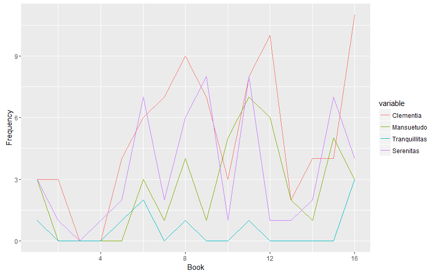
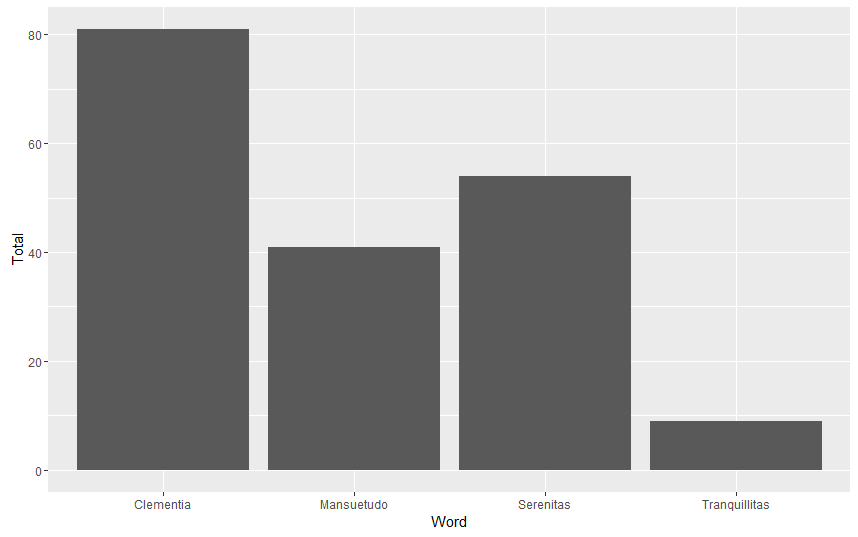
More immediately pertinent may be the sheer total number occurrences of each title within the Theodosian Code. Of the terms searched, Nostra Clementia is clearly the most common; this is understandable, for the emperor’s clemency was often invoked in his capacity as supreme legislator and judge.

rplot


I intend to continue to run searches for other imperial titles, both within the Theodosian Code, and in other texts. Once I have perfected my coding, it will be easy to replicate. The one major issue with which I am still faced, however, is the fact that word order matters little in Latin, and while I have found all of the instances of Nostra Clementia and Clementia Nostra, there are instances within the Code where other words are interposed between Nostra and Clementia. For example:

capture


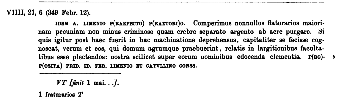
The phrase nostra scilicet super eorum nominibus edocenda clementia, “Our Clemency certainly ought to be informed of their names”, interposes the rest of the clause between nostra and clementia. I still need to figure out how to get R to find these instances and include them in my counts.


Code

CTh.scan <- scan(“~/Education/Emory/Coursework/Digital Humanities Methods/Project/Theodosian Code Raw Text.txt”,
what=”character”, sep=”\n”)
CTh.df <- data.frame(CTh.scan, stringsAsFactors=FALSE)
CTh.df <- str_replace_all(string = CTh.df$CTh.scan, pattern = “[:punct:]”, replacement = “”)
CTh.df <- data.frame(CTh.df, stringsAsFactors = FALSE)
CTh.lines <- tolower(CTh.df[,1])
book.headings <- grep(“book”, CTh.lines)
start.lines <- book.headings + 1
end.lines <- book.headings[2:length(book.headings)] – 1
end.lines <- c(end.lines, length(CTh.lines))
CTh.df <- data.frame(“start” = start.lines, “end”=end.lines, “text”=NA)
i <- 1
for (i in 1:length(CTh.df$end))
{CTh.df$text[i] <- paste(CTh.lines[CTh.df$start[i]:CTh.df$end[i]], collapse = ” “)}

CTh.df$Book <- seq.int(nrow(CTh.df))

CTh.df$Clementia <- str_count(string = CTh.df$text, pattern =
“nostra clementia|clementia nostra|nostrae clementiae|clementiae nostrae|nostram clementiam|clementiam nostram”)

CTh.df$Mansuetudo <- str_count(string = CTh.df$text, pattern =
“nostra mansuetudo|mansuetudo nostra|nostae mansuetudinis|mansuetudinis nostrae|
nostrae mansuetudini|mansuetudini nostrae|nostram mansuetudinem|mansuetudinem nostram|
nostra mansuetudine|mansuetudine nostra”)

CTh.df$Tranquillitas <- str_count(string = CTh.df$text, pattern =
“nostra tranquillitas|tranquillitas nostra|nostrae tranquillitatis|tranquillitatis nostrae|
nostrae tranquillitati|tranquillitati nostrae|nostram tranquillitatem|tranquillitatem nostram|
nostra tranquillitate|tranquillitate nostra”)

CTh.df$Serenitas <- str_count(string = CTh.df$text, pattern =
“nostra serenitas|serenitas nostra|nostrae serenitatis|serenitatis nostrae|nostrae serenitati|serenitati nostrae|
nostram serenitatem|serenitatem nostram|nostra serenitate|serenitate nostra”)

frequency.long <- melt(CTh.df, id = “Book”, measure = c(“Clementia”, “Mansuetudo”, “Tranquillitas”, “Serenitas”))
ggplot(frequency.long, aes(Book, value, colour = variable)) + geom_line() + ylab(“Frequency”) #Create Frequency Graph
clementia.sum <- sum(CTh.df$Clementia)
mansuetudo.sum <- sum(CTh.df$Mansuetudo)
tranquillitas.sum <- sum(CTh.df$Tranquillitas)
serenitas.sum <- sum(CTh.df$Serenitas)
Total <- c(clementia.sum, mansuetudo.sum, tranquillitas.sum, serenitas.sum)
Word <- c(“Clementia”, “Mansuetudo”, “Tranquillitas”, “Serenitas”)
word.sum.df <- cbind.data.frame(Word, Total)
ggplot(data=word.sum.df, aes(x=Word, y=Total)) + geom_bar(stat = “identity”) #Word Total Graph


Analyzing Heroin and Cocaine Arrest Patterns in Virginia:1971-1974

An overview of Heroin and Cocaine Arrests in virginia 1971-1974

vadrugbubbles
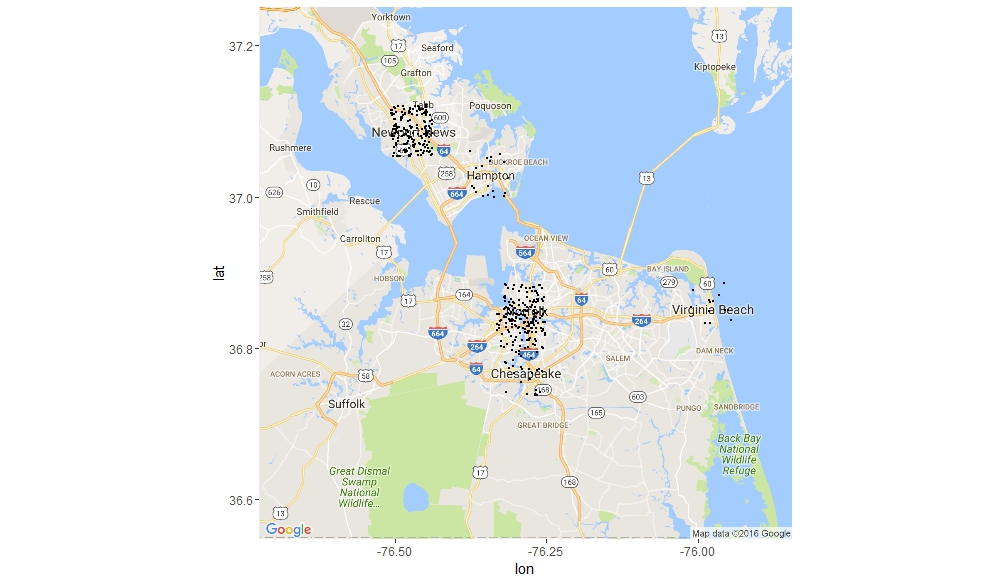
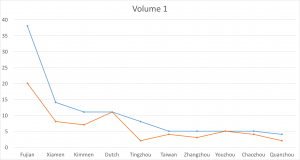
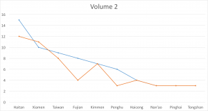
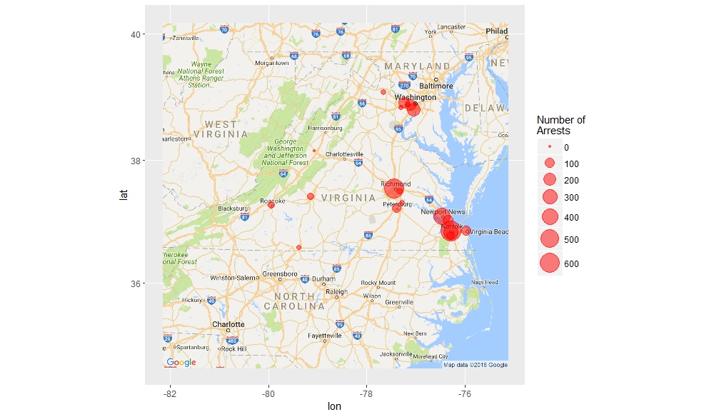
Tracking the Arrest Trends of the Five Localities with the Highest Volume of Arrests

cities
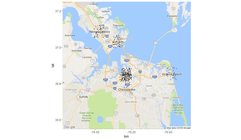
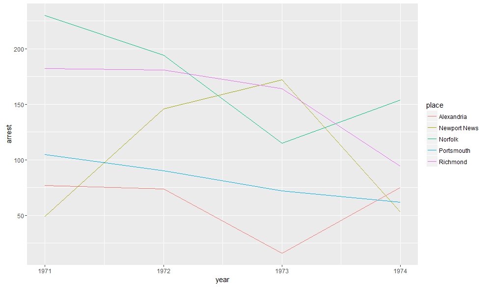
Richmond and Norfolk

norfolkrichmond
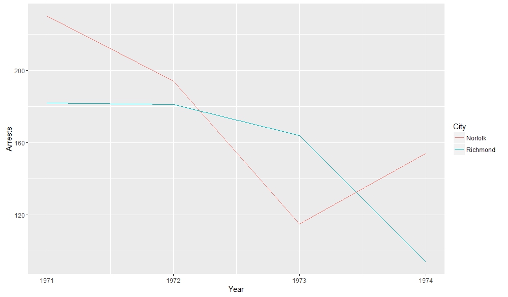
A Closer Reading of the Relationship Between Norfolk and Richmond

1972-heroin-shortage-in-norfolk-causes-users-to-buy-in-richmond-page-001


Tidewater Dot Maps

Study of Laughter in Works of Dazai Osamu

Background

Dazai Osamu (太宰 治) is a 20th-century Japanese novelist. Many of his works centers around mental illness and darkness of human nature, emitting abject or even morbid emotions. His most famous work include Run, Melos! (走れメロス)The Setting Sun, (斜陽) and No Longer Human, (人間失格). He committed suicide in 1948.

The text comes from Aozora Bunko (青空文庫), which is the Japanese Project Gutenberg. I downloaded the txt form of the works, but it is not cleaned as the txt from Project Gutenberg. I have to take out the ruby (inside《》, 笑《わら》う), Japanese pronunciation notation , the notation of the editor (inside[],[#「ファン」に傍点]), and “|” for separation in various conditions.

After cleaning these notation and white space, I first made a character frequency table of Ningen Shikkaku (No Longer Human). I admit I did this manually, chopping the text into single characters and kana, making the frequency table and deleting all kana. If there is a regex expression for kana in R, it will make this work easier.

Here is the first 25 most frequent character in Ningen Shikkaku

freq

One thing I find intriguing thing about this table is that in such a morbid and hopeless novel like Ningen Shikkaku, Dazai Osamu used the character for laugh (笑) for 103 times, 22nd of all characters.  This lead me to look closely into the character and possible vocabularies and conjugations that it forms.

Challenge of Tokenization

The challenge is tokenization. There are many great tools available online, but it takes time to learn to use them, and I do not know if they will work with long text. Therefore, for this week’s text, I used simple code to divide characters and kana into groups of same length. This does not directly solve the problem of tokenization, but rather goes around it.

Here is an example of the code for creating groups of length 2:

g2 <- 2
Text.cleaned.split.group2 <- paste(Text.cleaned.split[1:2], collapse = "")
     for (g2 in 2:(length(Text.cleaned.split) - 1)){
     group2 <- paste(Text.cleaned.split[g2:(g2+1)], collapse = "")
     Text.cleaned.split.group2 <- c(Text.cleaned.split.group2,group2)
}

The code runs so slowly, taking more than 10 seconds for a novel like Ningen Shikkaku. I am going to improve it if I am a better programmer. The same works for grouping of words in length three, four and five, but just runs even slower. For a rough text mining, group of words into length one, two or three should be enough.

The groups with length one, two, three are named

Text.cleaned.split.group1
Text.cleaned.split.group2
Text.cleaned.split.group3

I looked closely into the word formed with laugh (笑). First find every of incidence of character of 笑 in length one.

笑 <- grep(pattern = "笑", Text.cleaned.split.group1)

The start with some initial combination of length two like, 笑う,笑っ, 笑顔, 苦笑, 嘲笑, and find their positions in a vector variable called 笑.two.all. Use setdiff function to find remaining combinations of length two, adding them to my list. Here is an example:

笑う <- grep(pattern = "笑う", Text.cleaned.split.group2)
笑っ <- grep(pattern = "笑っ", Text.cleaned.split.group2)
笑顔 <- grep(pattern = "笑顔", Text.cleaned.split.group2)
嘲笑 <- grep(pattern = "嘲笑", Text.cleaned.split.group2) + 1L
笑.two.all <- c(笑う,笑っ,嘲笑,笑顔)
笑.others <- setdiff(笑,笑.two.all)

At the end, I come up with a list of 21 possible combinations in 16 works of Dazai Osamu :

笑う,笑い,笑っ,笑わ,笑む,笑声,失笑,笑ん,笑話,微笑,嘲笑,苦笑,笑顔,媚笑,可笑,一笑,の笑,笑え,憫笑,叟笑,笑お

When an author use the word laugh (笑), it is not always a positive word. We can have smile (微笑),  and laughing face (笑顔), but we also have to laugh at (嘲笑) and bitter laugh (苦笑).

Analyzing: positive or negative

My idea is to roughly group the combinations of length 2 into positive and negative laugh.

笑.two.positive <- c(笑う,笑い,笑っ,笑む,笑声,失笑,笑ん,微笑,笑顔,笑話,一笑,笑え,叟笑,笑お)
笑.two.negative <- c(笑わ,嘲笑,苦笑,媚笑,憫笑)

I then did a word frequency bar graph of the positive and negative laughter in all 16 works of Dazai Osamu. I put them all in chronological order, because I want to find if there is a change in style of the use of word.

ggplot(Freq.novel.df,aes(x = reorder(type,-value), y= value, fill = color))+
 geom_bar(stat="identity",color="grey50",position = "dodge", width = 1) +
 xlab("Type") + ylab("") +
 scale_fill_manual(values=c("dodgerblue2","firebrick3"),guide = FALSE) +
 ggtitle("1948_6_Ningenshikkaku")

1934_11_romanekusu 1936_7_kyokonoharu 1939_3_ogonfukei 1939_4_joseito 1939_6_hazakuratomateki 1939_8_hachijuhachiya 1939_11_hifutokokoro 1940_5_hashiremerosu 1942_6_seigitobisho 1944_3_sange 1944_8_hanafubuki 1944_9_suzume 1945_4_chikusei 1945_10_pandoranohako 1947_7_shayo 1948_6_ningenshikkaku


After making this graphs I find that short stories are more likely to become outliers, because they do not use the word a lot. Here is a comparison of the four novels. As I expected, Ningen Shikkaku is the has the most negative use of laugh.

1942_6_seigitobisho 1945_10_pandoranohako 1947_7_shayo 1948_6_ningenshikkaku


Reflection

I can make more graphs with my data from this week. For example a scattor plot of line plot with a x-axis in chronological order. Refining my searching lexicon can provide better data.

I can also search for place names with words with my group2, since most place names are in two characters. If I try to map it, I expect to get an enormous cluster around cities like Tokyo.

Doing text mining in languages like Japanese is hard, but not impossible. The method that I used in this week’s post will become tedious as I refine my searching lexicon. I can, however, run the same code on as many texts as I want, if my laptop does not crash because the verbosity of my code.

Full code:

library(stringr)
library(ggplot2)
Read in the file
Text.df <- read.delim("D:/Google Drive/JPN_LIT/Dasai_Osamu/1948_6_Ningenshikkaku.txt", header = FALSE, stringsAsFactors = FALSE, encoding = "CP932")
Text.text <- paste(Text.df[,1],collapse = "")
Text.splited.raw <- unlist(str_split(Text.text, pattern = ""))
Text.splited <- str_replace_all(Text.splited.raw, "|", "") # Take out all "|"
###grep
## Take out ruby and style notation
# Find out where to start and end
start <- grep(pattern = "《|[", Text.splited)
end <- grep(pattern = "》|]", Text.splited)
from <- end + 1
to <- start - 1
real.from <- c(1, from)
real.to <- c(to, length(Text.splited))
CUT.df <- data.frame("from" = real.from, "to"= real.to,"text" = NA)
# Solve the situation when form > end
row <- 1
CUT.fine.df <- data.frame("from" = 0, "to" = 0, "text" = NA)
for(row in 1:length(CUT.df$from)){
 if(CUT.df$from[row] <= CUT.df$to[row]){
 CUT.fine.df<- rbind(CUT.fine.df, CUT.df[row,])
 }
}
i <- 1
for(i in 1:length(CUT.fine.df$from)){
 text <- Text.splited[CUT.fine.df$from[i]:CUT.fine.df$to[i]]
 CUT.fine.df$text[i] <- paste(text, collapse = "")
}
Text.cleaned.text <- paste(CUT.fine.df$text, collapse = "") #cleaned up text, without ruby and style notations.
Text.cleaned.split <- unlist(str_split(Text.cleaned.text, pattern = ""))
###Run Code if you want a cleaned txt of the text
###Change name if needed
# write.table(Text.cleaned.text,"shayo.txt",row.names = FALSE, col.names = FALSE)
## A simple word count here (All punctuation, white spaces in English or Japanese format)
Text.wordcount <- str_replace_all(Text.cleaned.split, "[:punct:]", " ")
Text.wordcount <- Text.wordcount[which(Text.wordcount != " ")]
Text.freq <- data.frame(table(Text.wordcount))
Text.freq.ord <- Text.freq[order(-Text.freq$Freq),]
### Run code if you want a wordcount table.
### Change name if needed
write.table(Text.freq.ord, "Shayo_freq.txt",row.names = FALSE, sep = "\t")
### Grouping according to character length
## Runs slowly. 
## Do not use unless necessary. Uncomment before use.
Text.cleaned.split.group1 <- Text.cleaned.split
g2 <- 2
Text.cleaned.split.group2 <- paste(Text.cleaned.split[1:2], collapse = "")
for (g2 in 2:(length(Text.cleaned.split) - 1)){
 group2 <- paste(Text.cleaned.split[g2:(g2+1)], collapse = "")
 Text.cleaned.split.group2 <- c(Text.cleaned.split.group2,group2)
}
# g3 <- 2
# Text.cleaned.split.group3 <- paste(Text.cleaned.split[1:3], collapse = "")
# for (g3 in 2:(length(Text.cleaned.split) - 2)){
# group3 <- paste(Text.cleaned.split[g3:(g3+2)], collapse = "")
# Text.cleaned.split.group3 <- c(Text.cleaned.split.group3,group3)
# }
# 
# g4 <- 2
# Text.cleaned.split.group4 <- paste(Text.cleaned.split[1:4], collapse = "")
# for (g4 in 2:(length(Text.cleaned.split) - 3)){
# group4 <- paste(Text.cleaned.split[g4:(g4+3)], collapse = "")
# Text.cleaned.split.group4 <- c(Text.cleaned.split.group4,group4)
# }
#Word with length one
笑 <- grep(pattern = "笑", Text.cleaned.split.group1)
#Word with length two
笑う <- grep(pattern = "笑う", Text.cleaned.split.group2)
笑い <- grep(pattern = "笑い", Text.cleaned.split.group2)
笑っ <- grep(pattern = "笑っ", Text.cleaned.split.group2)
笑わ <- grep(pattern = "笑わ", Text.cleaned.split.group2)
笑え <- grep(pattern = "笑え", Text.cleaned.split.group2)
笑お <- grep(pattern = "笑お", Text.cleaned.split.group2)
笑む <- grep(pattern = "笑む", Text.cleaned.split.group2)
笑ん <- grep(pattern = "笑ん", Text.cleaned.split.group2)
笑顔 <- grep(pattern = "笑顔", Text.cleaned.split.group2)
笑話 <- grep(pattern = "笑話", Text.cleaned.split.group2)
笑声 <- grep(pattern = "笑声", Text.cleaned.split.group2)
微笑 <- grep(pattern = "微笑", Text.cleaned.split.group2) + 1L
嘲笑 <- grep(pattern = "嘲笑", Text.cleaned.split.group2) + 1L
苦笑 <- grep(pattern = "苦笑", Text.cleaned.split.group2) + 1L
媚笑 <- grep(pattern = "媚笑", Text.cleaned.split.group2) + 1L
可笑 <- grep(pattern = "可笑", Text.cleaned.split.group2) + 1L
一笑 <- grep(pattern = "一笑", Text.cleaned.split.group2) + 1L
憫笑 <- grep(pattern = "憫笑", Text.cleaned.split.group2) + 1L
叟笑 <- grep(pattern = "叟笑", Text.cleaned.split.group2) + 1L # For北叟笑む
失笑 <- grep(pattern = "失笑", Text.cleaned.split.group2) + 1L
の笑 <- grep(pattern = "一笑", Text.cleaned.split.group2) + 1L # This is the case when 笑 stands alone
# #Word with length three (uncomment before use)
# 笑われ <- grep(pattern = "笑われ", Text.cleaned.split.group3)
# 笑わせ <- grep(pattern = "笑わせ", Text.cleaned.split.group3)
# 
# #Word with length four(uncomment before use)
# 笑いませ <- grep(pattern = "笑いませ", Text.cleaned.split.group4)
笑.two.all <- c(笑う,笑い,笑っ,笑わ,笑む,笑声,失笑,笑ん,笑話,微笑,嘲笑,苦笑,笑顔,媚笑,可笑,一笑,の笑,笑え,憫笑,叟笑,笑お)
笑.two.positive <- c(笑う,笑い,笑っ,笑む,笑声,失笑,笑ん,微笑,笑顔,笑話,一笑,笑え,叟笑,笑お)
笑.two.negative <- c(笑わ,嘲笑,苦笑,媚笑,憫笑)
笑.two.neutral <- c(可笑,の笑) 
笑.others <- setdiff(笑,笑.two.all)
##### Graph Section of the code
###笑 divided positive and negative as frequecy in the novel
postive.freq <- length(笑.two.positive) / length(Text.wordcount)
negative.freq <- - length(笑.two.negative) / length(Text.wordcount)
Freq.novel.df <- data.frame ("type"= c("Positive", "Negative"), "value" = c(postive.freq,negative.freq),color = c("1","2"))
Freq.novel.df$type <- as.character(Freq.novel.df$type)
ggplot(Freq.novel.df,aes(x = reorder(type,-value), y= value, fill = color))+
 geom_bar(stat="identity",color="grey50",position = "dodge", width = 1) +
 xlab("Type") + ylab("") +
 scale_fill_manual(values=c("dodgerblue2","firebrick3"),guide = FALSE) +
 ggtitle("1948_6_Ningenshikkaku")

Does the Manchu matter? The Comparison of Ping Ding Hai Kou Fang Lue in Chinese and Manchus

1.   Introduction, Historiography, and Methodology

Is the Manchu language source merely the copy of Chinese source? Does the Manchu language source matter for studying Qing history? The question has been debated for over one century. In this article, I propose to argue that the Manchu language source not only matters but also is at least equally important as Chinese sources.

The oral Manchu language was used by Northeastern China, as known as Manchuria. In 1587, Nurgaci established a regime, and became khan of this area in 1589. In 1616, Nurgaci created a national title, Jin. During this period, because the government requested a more systematic writing so as to enhance the political efficiency, Erdeni and G’agai created the Manchu language based on the Mongolian linguistic system. This Manchu language writing system had limitation to spell non-Manchu language names or places, and, the most importantly, this writing system could not distinguish the sound k, g, and h. Comparing to the later revised Manchu language, this writing system was called the Old Manchu language.

In 1632, Hong Taiji, Nurgaci’s son, asked Dahai to modify the Old Manchu language. The new writing system included ten new words in order to spell names and places, clarified the difference between k, g, and h, and standardized the writing system. Therefore, for about 30 years, the Manchu language was mature enough to become a standard language to use. When the Qing occupied China, the Manchu language became the official language for all regions within the empire, including China, Mongolia, Tibet, and Uyghur until 1911.

In the early 20th century, Japanese scholars had noticed the importance and specialty of the Manchu language. Using the Manchu language sources to study Qing history had become more and more important in Japan. On the contrary, in China, although some scholars understand the Manchu language, using the Manchu language sources to study Qing history did not become a primary research approach at all. There are at least three main reasons.

First, because of Sinization, a lot of scholars did not pay attention on the Manchu language. For these scholars, in the same document, the Manchu language part was just translated from the Chinese part. Second, the amount of Chinese sources is the way more than the amount of the Manchu language sources. As a result, it is not necessary to read the Manchu language. Third, for them, the Manchu language was likely less important after the High Qing, and, meanwhile, ministers’ capacity of using Manchu language had gradually disappeared. As a result, because of these three reasons, the Manchu language sources had not been emphasized for a long time.

In 2004, a new historiographic approach appeared. This historiographic approach is called the New Qing History or the New Qing Imperial History. Over all, the New Qing History proposes to understand Qing history based on three new concepts. First, the New Qing History refuses the Sino-centrism, but, must be clarified, the New Qing History also does not entirely ignore the importance of Sinization. Instead of Sinicization, the New Qing History emphasizes the Manchu elements of the Qing Empire. Second, since the Qing Empire was not a Sinicized empire, the Qing Empire must have its unique. In this context, the New Qing History notices that the Qing Empire was in fact an empire as same as other empires in early modern period, such as the British Empire, Russia Empire, and Ottoman Empire. In other words, the Qing Empire was not a Chinese Empire but a universal empire, and China was just a part of this empire. Third, since the New Qing History emphasizes the importance of the Manchu element, the most direct approach to engage with the Manchus is widely using the Manchu language sources. For the New Qing historians, the Manchu language source is independent instead of a translation copy of Chinese part. Admittedly, the New Qing History generates considerable meaningful results and works, but increasing opponents still judge the three main concepts. One of the most common comments is that the New Qing historians overemphasize the importance of the Manchu language sources in an exaggerative way.

Based on this historiographic debate, this article analyzes a text in Chinese and the Manchu language. The text is Ping Ding Hai Kou Fang Lue (the Book of Strategic Record about Suppressing the Pirate, 平定海寇方略). Fang Lue was a literal form in the Qing period, and this form was only used by the government. When the Qing Empire defeated an enemy, the government edited a book for recording every detail chronologically based on official archives. Because Fang Lue was not only a book recording historical events but also a book proclaiming imperial victory, authority, and prestige, it is reasonable that the book should be edited in to multiple languages. So far, as we known, there were 25 Fang Lue. Among these 25 Fang Lue, Ping Ding Hai Lou Fang Lue was the only one which had not been found the completed version. In the past century, the Chinese version of this Lang Lue was the only version. Noticeably, this Chinese version was just a draft with four volumes. In 2011, I discovered the Manchu language version in the Grand Council Archive. This Manchu language version was also a draft, and it only had the first three volumes. Even though the Manchu volume only included the first three volumes, the Chinese version and the Manchu language version were still comparable because of three reasons. First, they overlapped the first three volumes. Second, they were edited at the same time. Third, they recorded the same event. Therefore, by comparing these two texts, this article seeks the relationship between the Chinese and the Manchu language versions.

As can be seen in Table 1, the Manchu and Chinese texts cover the exactly same period. In other words, these two texts record same events. In fact, this makes sense. Since the main purpose of this book is to record history and proclaim imperial prestige, the two texts should therefore have the same content. However, since the two texts should be in literal the same, it is interesting if there is any tiny difference.

Table 1: The period covered in the first three volumes

  Time Chinese source Manchu language source
Volume 1 Beginning March 1679 March 1679
End December 1679 December 1679
Volume 2 Beginning March 1680 March 1680
End August 1680 August 1680
Volume 3 Beginning March 1681 March 1681
End November 1682 November 1682


This article uses digital analysis to do text mining. The first problem encountered is the difference between two languages in grammar, writing system, and meaning. Because Chinese and the Manchu language are linguistically different, it is difficult, or impossible, to compare words by words. Fortunately, as mentioned above, since the two texts records the same events based on the same sources during the same time, the amount of the proper nouns and the name of places had to be matched. As a result, I propose to compare the amount of the name of places in two texts to see whether the two texts were translated or copied from the other. Then, I seek to individually map the name of places mentioned in two texts, and, by combining the geographic, political, and environmental phenomenon, I try to look for a big picture regarding the difference of the two texts.

2.   The Comparison of Two Texts

Table 2 suggests that, besides the term of “Dutch,” the rest name of places appeared more frequent in the Manchu language than in Chinese sources in the volume 1. It is hard to say whether the Manchu language text is more precise than Chinese text. However, this suggests that the Manchu language text and Chinese text are different. Table 3 suggests that the frequency of name of places in the Manchu language text is more than in the Chinese text. Nevertheless, the frequency of Kimmen, Nan’ao, Pinghai, and Tongshan are the same in both language texts. As a result, the two texts are different.

Table 2: The Frequency of the name of places in the Volume 1

Order Name of places Manchu texts Frequency Chinese texts Frequency
1 Fujian fugiyan 38 福建 20
2 Xiamen hiya men 14 廈門 8
3 Kimmen gin men 11 金門 7
4 Dutch ho lan 11 荷蘭 11
5 Tingzhou ting jeo 8 汀州 2
6 Taiwan tai wan 5 臺灣 4
7 Zhangzhou jang jeo 5 漳州 3
8 Youzhou yo jeo 5 岳州 5
9 Chaozhou coo jeo 5 潮州 4
10 Quanzhou ciowan jeo 4 泉州 2

Table 3: The Frequency of the name of places in the Volume 2

Order Name of places Manchu texts Frequency Chinese texts Frequency
1 Haitan hai tan 15 海壇 12
4 Xiamen hiya men 10 廈門 11
5 Taiwan tai wan 9 臺灣 8
9 Fujian fugiyan 8 福建 4
3 Kimmen gin men 7 金門 7
8 Penghu peng hū 6 彭湖 3
2 Haicheng hai ceng 4 海澄 4
6 Nan’ao nan oo 3 南澳 3
7 Pinghai ping hai 3 平海 3
10 Tongshan tung šan 3 銅山 3

Comparing to the previous two volumes, Table 4 shows a different result. Besides the Taiwan, Fujian, and Penghu, the rest of frequency is the same. However, it is apparent that frequencies of Taiwan and Fujian in the Manchu language text are more than in Chinese. Although the texts in the Manchu language and Chinese are slightly different, in terms of name of places, most of them are the same in the volume 3.

Table 4: The Frequency of the name of places in the Volume 3

Order Name of places Manchu texts Frequency Chinese texts Frequency
1 Taiwan tai wan 19 臺灣 11
3 Fujian fugiyan 16 福建 12
2 Penghu peng hū 8 彭湖 7
4 Kimmen gin men 3 金門 3
5 Xiamen hiya men 3 廈門 3
7 Zhejiang jegiyang 2 浙江 2
8 Pingyang ping yang 2 平陽 2
6 Haicheng hai ceng 1 海澄 1
9 Tongshan tung šan 1 銅山 1
10 Yungxia yūn siyoo 1 雲霄 1

Since I have compared the frequency of name of places in the first three volumes, it is obviously that the two texts are different. Although the difference is slight, they are different. Therefore, the Manchu language text or Chinese text are not the translated or copy version from the other. Using diagram is an appropriate approach to see how different the two texts are.

Graph 1: The line-graph of the difference in the Volume 1
20160929_blog_graphs_1
Graph 2: The line-graph of the difference in the Volume 2

20160929_blog_graphs_2

Graph 3: The line-graph of the difference in the Volume 3

20160929_blog_graphs_3

As can be seen, Graph 1, Graph 2, and Graph 3 suggest that the two texts are different in the most frequent name of places. In other words, the more frequent places are mentioned in text, the more different they are. When a place where are mentioned only few times in either text, this suggests that this place was only becoming significant at a certain moment or event during this period. For example, in the volume 2, Nan’ao, Pinghai, and Tongshan were mentioned only because a minister listed certain places where should be garrisoned. Besides this suggestion, these places were not important; to be specific, they should not be mentioned because they were not even the territory of the Qing Empire due to the Coastal Exclusion Policy. I will discuss this in the next section. Therefore, once the places were mentioned more frequent in the texts, they were highly different. In other words, I can confidently conclude that the two texts are different in terms of the frequency of name of places, even though they recorded the exactly the same period and event.

3.   A big picture of the geographical phenonmenon

In the previous section, I have left a question that the less frequent name of places should not appear due to the Coastal Exclusion Policy, but why were they still mentioned in two texts? This question might be able to answer when I incorporate the text mining with mapping together. According to the texts, the first sentence of the volume three addresses an important event. In the second month of the twentieth year of Kangxi Reign Period, the Qing Empire decided to repeal the Coastal Exclusion Policy. In other words, the lands in coastal area abolished due to the Policy could be used by people and government. However, this policy in fact was not successful because a lot of people still returned to their hometown before the policy repealed. This was widely known in Fujian but not in other regions.

In other words, the records in the volume 1 and 2 were the events when the Coastal Exclusion Policy was processed. However, the volume 3 was the record after the Coastal Exclusion Policy just repealed. Therefore, I propose to combine the result of the volume 1 and 2 as one fact but keep the volume 3 as an individual fact to discuss the difference between two texts under the historical phenomenon.

As can be seen in Map 1, between the frontier of blue points and seashore, the coastal area was entirely abandoned by the Qing Empire, so the area was in literal not a part of the empire. Therefore, when I mix the result of text mining and the mapping, this might help to understand history well.

Map 1: The Coastal Exclusion Policy

20160929_blog_cep

Map 2 is drawn by combining Map 1 and the result of Table 2, but I erase the large unit of place, such Fujian and Dutch, because I could not identify them in the map. As can been seen, the cities mentioned in text were almost beyond the front line, besides one point, which was Youzhou. In other words, from 1679 and 1680, the most frequent discussion about places located on the area where was belonged to neither the Qing nor the Zheng. By using the similar approach, Map 3 shows the result of Table 3 in the map.

Map 2: The frequency of places in the Manchu language in the volume 1 and 2

20160929_blog_volume12_m

Map 3: The frequency of places in Chinese in the volume 1 and 2

20160929_blog_volume12_c

Combining Map 1, Map 2, and Map 3, we could gain Map 4. It is interesting the difference between the Manchu language and Chinese sources in the map. Since the Manchu language mentioned these areas, where were not a part of the Qing, more direct than in Chinese, this is probably meaningful. Considering the feature and audience of the Manchu language, the Qing government probably did not allow Chinese general public, who could easily access to Chinese but the Manchu language, to understand details of the failure of the Coastal Exclusion Policy. In other words, this difference might imply how the empire control people’s mind and recognition of the true history.

Map 4: The frequency of places in the Manchu language and Chinese in the volume 1 and 2 under the map of the Coastal Exclusion Policy

20160929_blog_volume12_b

What was happened and changed when the Coastal Exclusion Policy was repealed? In fact, although the government prohibited people to return these abandoned areas, increasing people still returned where they settled before the policy processed. As a result, the policy was in reality useless. When the policy was repealed in 1681, people could return their original hometowns and lands. According to the previous discussion, if it is true that the reason to mention cities in abandoned area in Chinese less frequent and direct than in the Manchu language is because the government attempted to control people’s understanding, Map 5, Map 6, and Map 7 could exactly interpret why the two texts are similar in the volume 3. Because the Coastal Exclusion Policy had been repealed, it was not necessary to hide from anything about the fail of Coastal Exclusion Policy.

Map 5: The frequency of places in the Manchu language in the volume 3

20160929_blog_volume3_m

Map 6: The frequency of places in Chinese in the volume 3

20160929_blog_volume3_c

Map 7: The frequency of places in the Manchu language and Chinese under the repealed Coastal Exclusion Policy

20160929_blog_volume3_b

Map 8 is mixed Map 1 to 7. It might suggest and support my argument in previous paragraph. Therefore, I can certainly be confident to argue that the Manchu language was more precise, detailed, and direct to mentioned the name of places than in Chinese because the government did not reveal the failure of processing the Coastal Exclusion Policy. Although the failure of the Coastal Exclusion Policy was widely known in Fujian, it was not recognized in other provinces and non-China regions, such as Mongolia and Tibet. Because the main purpose of editing this book is to proclaim the imperial prestige and success, the government had to carefully control the content. The threshold of learning the Manchu language was higher than learning Chinese because the Manchu language was only used in high class. In contrast with the Manchu language, Chinese had been the dominant language for over two thousand years. The failure of the Coastal Exclusion Policy could be limitedly recognized by ruling class, but this could not be known by Chinese folks.

Map 8: The frequency of places in the Manchu language and Chinese under the Coastal Exclusion Policy in the first three volumes

20160929_blog_volume123

4.   Conclusion

According to the approach of the digitial humanities, conducting text mining to compare two different languages of the same book suggests that the Manchu language or Chinese text was not the copy or translation version of the other. Moreover, the frequency of places in the Manchu language is slightly more precise than Chinese version. Moreover, because the historical background, the frequency of places in this book might be highly related to the imperial policy, the Coastal Exclusion Policy. In fact, combining the text mining and spatial history, it shows how the government controlled texts to limit folks to recognize the failure of the Coastal Exclusion Policy.

Admittedly, I can read the Manchu language and Chinese. Frankly, before I used the approach of the digital humanities to analyze these two texts, I believe that the two texts in fact were exactly the same although I’m a follower of the New Qing History, which means that I did not believe the Manchu language sources were translated from Chinese sources. However, in this case, for me, there was probably a main draft or main author, and the two texts were just edited from the main draft. However, because of the difference between the frequency of places, I change my mind. Also, this enhances the idea of the New Qing History: the Manchu language and Chinese sources should be equally emphasized in order to establish a broader Qing history.


Mixed Results with the Aeneid

Code A

I must confess to getting a bit of a late start on this week’s blog post (busy week), and as a result I have found myself stuck on a particular line of the chunking code that I have yet to trial-and-error my way through. The 12 book (read: chapter) divisions of the Aeneid are listed as “Liber I, Liber II, Liber III, etc.”, and I can’t quite get the grep function (which I admittedly still do not fully understand) to mark these headings. I believe that the line of code as I have it (bolded below) indicates the phrase “LIBER + (some combination of Roman numerals”, but even so R comes back with 23 hits instead of the expected 12.

What I had intended to do was to track the occurrences of “virtus” (~manly martial virtuous excellence) and “pius” (~reverent toward the gods and one’s family and duty), both of which are major themes in the Aeneid. Perhaps I will be able to do so once I figure out what’s tripping me up with the grep function. Again, apologies for not coming to Dr. Ravina with this sooner.

Aeneid.lines.scan <- scan(
“~/Education/Emory/Coursework/Digital Humanities Methods/RStudios Practice/Aeneid Raw Text.txt”,
what=”character”, sep=”\n”) # Scan Aeneid Raw Text

start.line <-
which(Aeneid.lines.scan==”PUBLI VERGILI MARONIS”)
end.line <- which(Aeneid.lines.scan==”vitaque cum gemitu fugit indignata sub umbras.”)

poem.lines <- Aeneid.lines.scan[start.line : end.line]
book.headings <- grep(“^[LIBER I|V|X]*$”, poem.lines)
start.lines <- book.headings + 1

end.lines <- book.headings[2:length(book.headings)] – 3
end.lines <- c(end.lines, length(poem.lines))

Aeneid.df <- data.frame(“start” = start.lines, “end”=end.lines, “text”=NA)
i <- 1
for (i in 1:length(Aeneid.df$end))
{Aeneid.df$text[i] <- paste(poem.lines[Aeneid.df$start[i]:Aeneid.df$end[i]], collapse = ” “)} View(Aeneid.df)
Aeneid.df$virtus <-
str_count(string = Aeneid.df$text, pattern = “\\Wvirtus\\W|\\WVirtus\\W”)

Aeneid.df$book <- seq(1,12,1)
plot(Aeneid.df$book, Aeneid.df$virtus)

Aeneid.df$pius <-
str_count(string = Aeneid.df$text, pattern = “\\Wpius\\W|\\WPius\\W”)

Aeneid.df$book <- seq(1,12,1)
plot(Aeneid.df$book, Aeneid.df$pius)

Code B

I had more success dealing with the KWIC analysis (although I should point out that in both this and the previous set of coding, I am still hampered by my ignorance of stemming and NLTK for Latin. Here I looked at the context in which one found the word “pius” with either “Aeneas” (to whom the epithet is often given) or “At” (meaning “but”, and something that I noticed appeared in a number of lines with “pius”).

poem.total <- paste(poem.lines, collapse=” “)
length(poem.total)

nchar(poem.total)

poeml.total <- tolower(poem.total)

poem.words <- unlist(str_split(poem.total, “\\W”))
length(poem.words)

poem.words <- poem.words[which(poem.words!=””)]
length(poem.words)

locations.kwic <- which(poem.words==’pius’)
start.kwic <- locations.kwic – 5
end.kwic <- locations.kwic + 5
start.kwic <- ifelse(start.kwic>0, start.kwic, 0)
end.kwic <- ifelse(end.kwic<length(poem.words),
end.kwic, length(poem.words))

KWIC.df <- data.frame(“start” = start.kwic, “end” = end.kwic, “text” = NA)

i <- 1
for (i in 1:length(KWIC.df$start)){
text <- poem.words[KWIC.df$start[i]:KWIC.df$end[i]]
KWIC.df$text[i] <- paste(text, collapse = ” “)
}

view(text)

index.no <- which(poem.words==’pius’)
context.count <- str_count(KWIC.df$text, “Aeneas|At”)
plot(index.no, context.count)

rplot

Comparison of Two Plantation Narratives

For this week’s blog post, I decided to rerun the same code as last week but on two different texts: (1) James B. Avirett’s The Old Plantation: How We Lived in Great House and Cabin Before the War and (2) Charles Ball’s Fifty Years in Chains, or, The Life of an American Slave. These books are part of the “First-Person Narratives of the American South” Collection at the University of North Carolina-Chapel Hill’s Documenting the American South website. Both of these books provide narratives showing different perspectives of plantation life.

James Battle Avirett was born on a plantation in Onslow County, North Carolina ca. 1837. He grew up in the antebellum South and became an ardent defender of its traditions. Charles Ball’s story, on the other hand, reflects his experience growing up on a tobacco plantation in Calvert County, Maryland. Ball’s book should be interesting to compare with Avirett’s as it was written with the help of a man named Isaac Fischer. In his preface, Fischer declares that he has edited the oral narrative Ball dictated to him to omit any beliefs or feelings Ball may have expressed about slavery. Fischer’s editing should be evident in the word frequency analysis.


Below is a table with the most common words occurring in Avirett’s text that are not in the most common words of Ball’s text.

“Common Words in Avirett not in Ball”
“1” “is”
“2” “old”
“3” “their”
“4” “are”
“5” “you”
“6” “so”
“7” “have”
“8” “these”
“9” “out”
“10” “there”
“11” “plantation”
“12” “those”
“13” “what”
“14” “up”
“15” “large”

Below is a table with the most common words occurring in Ball’s text that are not in the most common words of Avirett’s text.


“Common Words in Ball not in Avirett”
“1” “i”
“2” “my”
“3” “me”
“4” “master”
“5” “him”
“6” “who”
“7” “our”
“8” “after”
“9” “her”
“10” “could”
“11” “time”
“12” “them”
“13” “no”
“14” “now”
“15” “two”
“16” “day”

Among some of the differences that stand out are Avirett’s more frequent use of “old,” plantation,” and “large” compared with Ball’s more frequent use of “master,” “him,” “time,” and “day.” While both books are personal narratives, it is interesting to note that Ball uses “I,” “me,” and “my” more often than Avirett, who more frequently uses “their,” “you,” “these,” and “those.

To take the analysis a step further, I plotted charts for both texts to show the frequency at which the word “master” occurs throughout each chapter.

avirett2

ball-master

Additionally, I plotted charts for both texts to show the frequency at which the word “master” occurs throughout each chapter.

avirett

ball-plantation

Comparing Word Usage in Shakespeare’s the Rape of Lucrece and Venus and Adonis

When William Shakespeare dedicated his narrative poem Venus and Adonis to his benefactor in 1593 he made a solemn promise. “I… vow to take advantage of all idle hours, till I have honoured you with some graver labour.” A year later he produced the Rape of Lucrece, a poem considered by many to be one of “the Bard’s” more serious works. Using the text mining tools in R we can see that Shakespeare appears to have fulfilled his vow. While there are numerous similar words that point to an unsurprising similarity in style(after all both were written in narrative form and back to back), the more distinctive words in each seem to illustrate a marked gap in the tone of these poems. The Rape of Lucrece  mentions words like “honour,” “sad,” and “sin,” more then Venus and Adonis. Comparatively, the latter makes use of more positive words like, “kiss,” “boar,” and “cheek.” Yet, context is all, and those of us who have read Venus and Adonis know that a “kiss” may not be enjoyed by all and the hunted may become the hunter. Thus, in a forthcoming post, we will delve deeper into these two works using R’s sentiment analysis tools and call Shakespeare to account for the vow he made 423 years ago.

The Comparison Table

Common Lucrece Distinctive Venus Distinctive Lucrece “More” Distinctive* Venus “More” Distinctive*
the which love honour kiss
and when now sad boar
to then shall sin boy
in have more while cheek
of such being live hard
his did heart thing best
*These categories exclude proper nouns

The code that makes it work

#First download Venus and Adonis and the Rape of Lucrece in .txt form, from PorjectGutenberg. You will also need the stringr and stringi packages.
##Part 1- Cleaning up “The Rape of Lucrece”
Lucrece.lines.scan<scan(“c:\\yourname\\location\\TheRapeofLucrece.txt”,what=”character”, sep=”\n”)
Lucrece.lines Lucrece.lines Lucrece.string Lucrece.words Lucrece.words Lucrece.words Lucrece.words.df Lucrece.words.df$lower colnames(Lucrece.words.df)[1]<- “words”
Lucrece.words.df$clean_text Lucrece.words.df$cleaned Lucrece.clean.tbl.df Lucrece.cleaned.tbl.ord.df colnames(Lucrece.cleaned.tbl.ord.df)[1] <- “Words”
#Cleaning up “Venus and Adonis
VenusAdonis.line.scan VenusAdonis.lines VenusAdonis.lines VenusAdonis.string VenusAdonis.words VenusAdonis.words VenusAdonis.words VenusAdonis.words.df VenusAdonis.words.df$lower colnames(VenusAdonis.words.df)[1]<- “words”
VenusAdonis.words.df$clean_text VenusAdonis.words.df$cleaned VenusAdonis.clean.tbl.df VenusAdonis.cleaned.tbl.ord.df colnames(VenusAdonis.cleaned.tbl.ord.df)[1] <- “Words”
#Part 2- Comparison
##Which words are common in both “the Rape of Lucrece” and “Venus and Adonis”?
table<-intersect(Lucrece.cleaned.tbl.ord.df$Words[1:10],VenusAdonis.cleaned.tbl.ord.df$Words[1:10])
write.table(table, “C:\\your.location\\VenusAdonis-Lucrece.csv”,sep=”,”, col.names=NA)
##Which words are “somewhat”distinctive?
setdiff(Lucrece.cleaned.tbl.ord.df$Words[1:50],VenusAdonis.cleaned.tbl.ord.df$Words[1:50])
setdiff(VenusAdonis.cleaned.tbl.ord.df$Words[1:50],Lucrece.cleaned.tbl.ord.df$Words[1:50])
##Which words are “more”distinctive?
VenusAdonis.cleaned.tbl.ord.df[which(!VenusAdonis.cleaned.tbl.ord.df$Words[1:500]%in% Lucrece.cleaned.tbl.ord.df$Words[1:500]),]
Lucrece.cleaned.tbl.ord.df[which(!Lucrece.cleaned.tbl.ord.df$Words[1:500]%in% VenusAdonis.cleaned.tbl.ord.df$Words[1:500]),]

Does the Manchu language matter?

Introduction

Do you still remember the text in the standard Manchu language, which is Ping Ding Hai Kou Fang Lui (The Book about Defeating Piracy, 平定海寇方略)? In this blog, I propose to briefly explain the background of editing this book, and I analyze and compare within this book. The most importantly, I analyze and compare the version of this book in two languages, Chinese and the Manchu language. By understanding this analysis, I argue that the Manchu language texts and Chinese texts are different and equally important to know.

During the Qing China (1644-1911), the Qing Empire had a tradition on editing book for detailing victory, and the form of this kind of books is “Fang Lue” in Chinese and “necihiyeme toktobuha bodogon i bithe” in the Manchu language. The main function of Fang Lue was for proclaiming how powerful and successful the Qing Empire was. In order to widely spread the success of the Qing Empire, Fang Lue usually edited in the Manchu language and Chinese, sometimes in other languages, such as the Mongolian.

Ping Ding Hai Kou Fang Lue was edited for recording the battle between the Qing Empire and the Zheng Regime in Taiwan, which was regarded as pirate for the Qing. The Zheng Regime was formally created by Zheng Chenggong, as known as Koxinga, during Ming Qing transition. However, Koxinga’s father, Zheng Zhilong, was the substantial founder of this regime in the later Ming Dynasty. Zhilong was originally a pirate as well as a trader, but he was recruited by the Ming government as an official general in Fujian, a southeastern province of China, so as to help the Ming Court to suppress other pirate in 1627.

After few years, in 1635, Zhilong successfully defeated the last resister. Due to Zhilong’s contribution during these years, Zhilong had been appointed as the commander of Fujian. Zhilong became the practical controller in Fujian. During Ming Qing transition, although Zhilong supported the Ming Court at the beginning, Zhilong eventually decided to surrender to the Qing Empire, but he did not bring all troops and property with him to Beijing.

Instead, Zhilong’s brothers and sons were still in Fujian with holding unbelievably powerful army and navy. Koxinga, Zhilong’s eldest son, was not the most powerful general in the Zheng Regime at this time, but, as a half Japanese and trained as a Japanese samurai and a Chinese Confucianist, Koxinga gradually nibbled up his relative’s troops and annexed their territory to enhance his power. Around 1650s, Koxinga had not only dominated the Zheng Regime but also become the most influential and powerful anti-Qing power in China.

However, in 1660, Koxinga misapprehended his capacity, so he attacked Nanjing City beside Yangzi River. Undoubtedly, he failed because of Koxinga’s arrogance and misstep. Next year, he led his navy and army to Taiwan. After one-year battle with the Dutch East India Company, Koxinga accepted Dutch’s surrender, and the Zheng Regime began to reign Taiwan as an anti-Qing basis. From 1661 to 1683, the Qing Empire and the Zheng Regime negotiated with each other to intend to find a balance to keep peaceful sphere. However, they never reached an agreement.

In 1683, Shi Lang, the former general of the Zheng Regime and the navy marshal of the Qing Empire at this time, defeated the Zheng Regime. As a result, Zheng Keshuang, the last king of the Zheng Regime, surrendered to the Qing Empire. This event was extremely important for the Qing Empire. First, the last anti-Qing power eventually vanished. Second, the Qing Empire occupied a new territory as its colony. Third, the Qing Empire could focus on the threat from the Inner Asia. This was the reason why this battle was worth to record as a Fang Lue.

The Ping Ding Hai Kou Fang Lue’s Manchu language version

There are 25 Fang Lues officially edited by the Qing Empire, and the form of Fang Lue is edited by chronological. However, among them, the Ping Ding Hai Kou Fang Lue was the only one which was not found the formal version in Chinese. In other words, it was a draft. For the past century, this version was the only one recognized, which had four volumes. In 2011, I’m the first person to discover the draft in the Manchu language although there were only first three volumes remaining.

First of all, I propose to compare the first and second volumes. As can be seen in Table 1, I list the frequent words in the volume 1 but not in the volume 2. Obviously, almost all frequent words in the volume 1 but not in the volume 2 are name of people or place. For example, the first is Fujian, which was the name of a province in southeastern China. Moreover, the second frequent word is wang, which refers to king. In other words, kings were not important in the volume 2. Additionally, ceng and gung refer to the same person, who is Koxinga, and jy and lung refer to Koxinga’s father, Zhilong. In other words, these two important people are not important in the volume two. The reason of less frequent names and places is because this Fang Lue was edited chronologically, so these places or people in the period described in the volume 2 are no longer essential.

Additionally, another noticeable difference between two volumes is that there are a lot of terms regarding the emperor, such as hese, dergi, hesei, and wasimbuhagge. Does this indicate that emperor is less important in the volume 2? Yes, it does. In fact, this perhaps addresses that the content of the volume 1 records the emperor’s orders, but the content of the volume 2 mainly records the discussion between ministers and generals as well as the battle between the Qing and the Zheng.

Table 1: comparing the difference in the first and second volume.

Order Words English meaning Frequency in Vol. 1 Frequency in Vol. 2
1 fugiyan Fujian 38 8
2 wang king/surname 36 3
3 ni of 34 7
4 gung (name of a person) 33 0
5 ceng (name of a person) 27 4
6 hese emperor’s order 23 7
7 manggi when… 23 7
8 aniya year 22 2
9 jy (name of a person) 22 0
10 lung (name of a person) 20 0
11 hebei discussion’s 19 1
12 sede speak 17 0
13 dergi east/up/Majesty 16 6
14 hesei of the emperor’s order 16 5
15 wasimbuhangge the order from emperor 16 3

Next, I compare the frequent words in the volume 1 and also in the volume 2.  As can been seen in Table 2. Besides the most frequent auxiliary words, the most frequent words usually referred to certain important people or place in both volumes, such as Wan Zhengse (wan, jeng, and še in the Manchu language), the most important general (tidu) during this period, and Quanzhou (cuwan jeo in the Manchu language), the most important area in Fujian.

Table 2: comparing the similarity in the first and second volume.

Order Words English meaning Frequency in Vol. 1 Frequency in Vol. 2
1 be be 242 126
2 de at 131 59
3 i of 127 67
4 jeng (surname) 81 23
5 cooha military/army 80 53
6 cuwan (name of a place) 49 21
7 mederi ocean 44 11
8 seme so/although 41 21
9 jeo prefecture 38 11
10 hūlha bandit 36 19
11 sehe spoke 28 14
12 wan (surname) 27 28
13 men (name of places) 25 19
14 tidu commander 25 24
15 fu (administrative level) 24 19
16 amba big 23 12
17 gin (name of a place) 22 11
18 še (name of a person) 22 19
19 dzungdu viceroy 21 16
20 dahame therefore 20 14

Table 3 suggests that the most frequent words in the volume 2 but not in the volume 3. Apparently, besides numbers (minggan, emu, juwe, and ilan) and gaimbi in different forms (gaifi and gaiha), the rest words are related to name of people or place. The question here is why gaimbi, referring to “get” in English, appears frequently. According to the content of the second volume, it primarily accounts the battle between two regimes, so it makes sense because gaimbi also refers to “occupy city” in English. As a result, the volume 2 in fact discusses how the cities in Fujian were occupied by turns.

Table 3: comparing the difference in the second and third volume

Order Words English meaning Frequency in Vol. 2 Frequency in Vol. 3
1 hai (name of a place) 26 1
2 men (name of places) 19 6
3 še (name of a person) 19 3
4 minggan thousand 15 0
5 tan (name of a place) 15 0
6 gaifi gotten 14 7
7 juwe Two 14 4
8 ilan three 13 3
9 emu one 12 6
10 gaiha got 11 0
11 gin (name of a place) 11 7
12 jeo prefecture 11 0
13 hafan officials 10 4
14 hiya guard 10 3
15 se etc. 10 7

Table 4 suggests the most similar words. Besides the auxiliary words, over half of the most frequent words in both volumes refers to name of place or people. However, noticeably, the surname, such as jeng and u is often the most frequent in both volumes. This actually indicates that in the Manchu language version, the author preferred to write entire name instead of only first name. This is in fact very different from the Chinese version, whose author preferred to write only first name.

Table 4: comparing the similarity in the second and third volume

Order Words English meaning Frequency in Vol. 2 Frequency in Vol. 3
1 be be 126 139
2 i of 67 54
3 de at 59 60
4 cooha military/army 53 38
5 wan (surname) 28 23
6 tidu commander 24 22
7 jeng (surname) 23 8
8 cuwan (name of a place) 21 14
9 seme so/although 21 22
10 amban minister 19 13
11 fu (administrative level) 19 16
12 hūlha bandit 19 16
13 u (surname) 19 8
14 siyūn governor 17 16
15 dzungdu viceroy 16 26
16 hing (name of a person) 15 9
17 dahame therefore 14 18
18 dzu (name of a person) 14 8
19 sehe spoke 14 22
20 gemu together 13 9

The comparison within this book suggests that each volume has its own emphasis because this book was edited chronologically. Especially, the similarity was usually about grammar and certain important places or people. Since the content of this book was edited chronologically, the difference implied where is much more important, who is much more important, and what is much more important for different periods.

The Comparison of the same text in the different language

As mentioned, for over one century, the Chinese version was the only recognized one. Since the new version in the Manchu language has been discovered, it is important to compare two versions.

However, noticeably, Chinese is hard to analyze as a systematical language. Since Chinese is an alphabetic system of writing, each Chinese character might have multiple meanings and multiple Chinese combined together will generate different meanings. Due to these features of Chinese characters, I would like to use a different way to analyze and compare two texts. First, I analyze the text in the Manchu language to recognize the frequency of each words. Then, I search the top 20 frequent words in Chinese version to see whether the frequency is similar. As a result, let’s search the most frequent words in Volume 1, 2, and 3 in the Manchu language version, and check out the frequency in the Chinese text.

Table 7: the comparison of the frequency of words in the volume 1

order Words Frequency English Chinese Frequency in Chinese version
1 be 242 be
2 de 131 at
3 i 127 of
4 jeng 81 (surname) 3
5 cooha 80 military/army 軍/兵 軍25/兵51
6 cuwan 49 (name of a place) 2
7 mederi 44 ocean 46
8 seme 41 so/ although
9 fugiyan 38 Fujian 福建 20
10 jeo 38 Prefecture 12
11 hūlha 36 bandit 賊/寇 賊17/寇20
12 wang 36 king 22
13 ni 34 of
14 gung 33 (name of a person) 14
15 sehe 28 spoke


Graph 1: The comparison of the frequency of words in the volume 1 as a line graph

figure_1

As can be seen, besides the terms which could not be found in Chinese, such as be, de, and i, in Manchu language, jeng, which was the surname referring to Zheng (鄭) in Chinese, rarely appeared in the Manchu text. Meanwhile, in the Manchu text, cuwan, referring to Quanzhou (泉州) in Chinese,  frequently appeared, but this word only appeared twice in the Chinese text. Also, in the Manchu text, fugiuan, referring to Fujian (福建) in Chinese, was almost double times more than this term in Chinese.

Table 8: the comparison of the frequency of words in the volume 2

order Words Frequency English Chinese Frequency in Chinese version
1 be 126 be  
2 i 67 of  
3 de 59 at  
4 cooha 53 military 軍/兵 軍19/兵64
5 wan 28 (surname)/Taiwan 萬/灣 萬14/灣19
6 hai 26 (name of a place) 12
7 tidu 24 commander 提督 32
8 jeng 23 (surname) 6
9 cuwan 21 (name of a place) 2
10 seme 21 so/although
11 amban 19 minister 36
12 fu 19 (administrative level) 0
13 hūlha 19 bandit 賊/寇 賊29/寇13
14 men 19 (name of places) 24
15 še 19 (name of a person) 18


Figure 2: The comparison of the frequency of words in the volume 2 as a line graph

figure_2

According to Table 8 and Graph 2, similarly, jeng in the Manchu text is almost four times more than Zheng in the Chinese text. Also, cuwan, fu, and hai were more frequent in the Manchu text than in the Chinese text.


Table 9: the comparison of the frequency of words in the volume 3

order Words Frequency English Chinese Frequency in Chinese version
1 be 139 be
2 de 60 at
3 i 54 of
4 cooha 38 military/army 軍/兵 軍16/兵68
5 dzungdu 23 viceroy 總督 7
6 ki 23 (name of a person) 10
7 šeng 23 (name of a person) 10
8 wan 23 Taiwan 29
9 yoo 23 (surname) 6
10 sehe 22 spoke
11 seme 22 so/although
12 tidu 22 commander 提督 20
13 ši 19 (surname) 25
14 tai 19 Taiwan 29
15 dahame 18 therefore 3

Graph 3: The comparison of the frequency of words in the volume 3 as a line graph

figure_3

As can be seen, Table 9 and Graph 3 suggest that name of places or people were more complete in the Manchu text than Chinese text. This is also apparent in the volume 1 and volume 2.

The Manchu language and Chinese are extremely different languages. The Manchu language is belonged to Altaic language and syllabary, just like Japanese. Instead, Chinese (Mandarin) is belonged to Sino-Tibetan language and logogram. Therefore, it is hard to compare the frequency of each word in two texts. However, certain words, especially nouns, are still comparable.

This comparison is meaningful because this comparison is related to a debate between the New Qing History and its opponents. For a long time, Chinese sources have been the dominant sources to study Qing history. For these scholars, primarily the opponents of the New Qing History, the Qing Empire was not an empire; in the lieu of an empire, the Qing was entirely incorporated by Chinese culture and system, so the Qing was actually one of Chinese dynasties. This perspective was called Sinicization. In order to support their idea regarding Sinicization, they claimed that all texts written in the Manchu language was just the copy of the Chinese version, so the versions in the Manchu language were meaningless because scholars could directly read Chinese version.

Is this correct? Let’s look the new graphs, which are modified from Graph 1, 2, and 3. They are Graph 4, 5, and 6. The main difference between Graph 1, 2, 3 and Graph 4, 5, 6 is that I omit the term in the Manchu language but not in Chinese, for example auxiliary words. The reason is not because these terms do not exist in Chinese but they exist in the thousand possibilities in Chinese, so it is difficult to define which words in the Manchu language directly refer the words in Chinese; otherwise, I do a carefully reading.

Graph 4: the terms in both texts in volume 1

figure_1without-noncharacter

Graph 5: the terms in both texts in volume 2

figure_2without-noncharacter
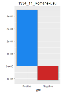
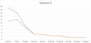
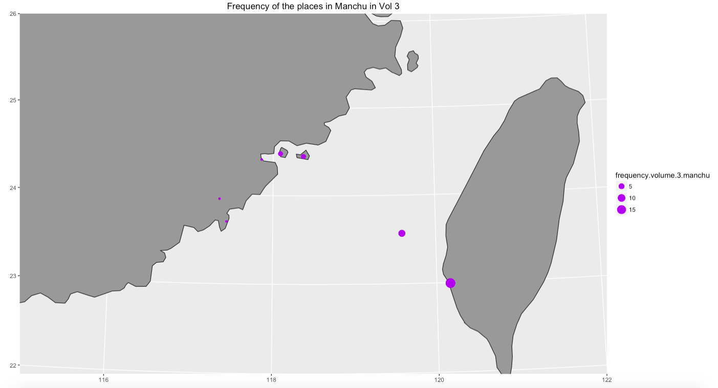
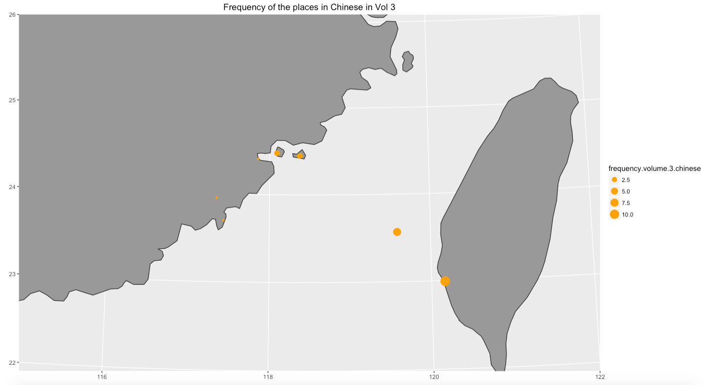
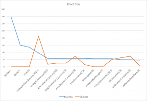
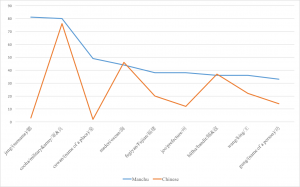
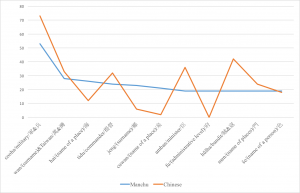
Graph 6: the terms in both texts in volume 3

figure_3without-noncharacter

Do you notice anything? The answer is quite obvious. Even though the same nouns, usually place or people’s name, appeared in both texts, their frequencies are still significantly different. Can the opponents of the New Qing History insist to claim that the Manchu language versions were just the copy of the Chinese version? I do not think so.

Conclusion

Admittedly, it is not sure whether this comparison is meaningful, but it does suggest a general idea. The idea is that the Manchu text was usually more precise than the Chinese text. However, in other words, Chinese can be more laconic. As a result, this might imply that the Manchu language was still less mature than Chinese, in some degree.

Apparently, there is a big question waiting for answering. Let’s look at Table 7, 8, and 9. Some terms, such as tidu, fugiyan, dzungdi, and so on, directly referred to a certain place or people. However, why were the number of these terms in the Manchu and Chinese texts different? According to the comparison and graphs, the Manchu language version and Chinese version were in effect different. Neither one was just the copy of another version. They were equally important but addressed to different audience and purpose.

Consequently, since this comparison had offered a general picture, the next step might be to do a closed reading to come up with the answer for the detail difference between the text in two languages.

Using R to Compare Word Frequencies in Two of Shakespeare’s Comedies

R is a “free software environment for statistical computing and graphics” that can be used for text mining. For this blog post, I have used R to create tables of word frequencies in two of Shakespeare’s comedic plays: The Comedy of Errors and The Tempest.

The first page of Shakespeare’s The Comedy of Errors, printed in the First Folio of 1623 (Wikimedia Commons / Folger Shakespeare Library Digital Image Collection)

Below is a table showing the ten most frequent words occurring in Shakespeare’s The Comedy of Errors. Not surprising, some of the most common words are prepositions (of, to), articles (the, a), and a conjunctions (and). The first person pronoun “I” occurs about 1.5 times more frequently than the second person pronoun “you.” This correlates with the book’s story of the unwitting encounters between the lost twin sons (both named Antipholus) and their twin servants (both named Dromio). The most common noun, “Syracuse,” indicates a place in the story.

WORDS FREQUENCY
“of” 612
“and” 465
“I” 461
“the” 448
“to” 335
“you” 302
“my” 265
“me” 262
“a” 244
“Syracuse” 234
Title page of The Tempest from the 1623 First Folio (Wikimedia Commons / The Internet Shakespeare Editions)

The most common words in The Tempest are not that different from The Comedy of Errors. Again, we mostly see conjunctions, articles, and prepositions. The first person pronoun “I” occurs 2.5 times as often as the second person “you” as Shakespeare tells the story from the point of view of the magician Prospero, a former duke of Milan exiled on an island, where is accompanied by his daughter, Miranda, the spirit Ariel, and the monster Caliban.

WORDS FREQUENCY                         
“and” 525
“the” 457
“I” 453
“to” 324
“of” 304
“a” 301
“my” 287
“you” 209
“that” 193
“this” 186

Now, let’s see how the two texts differ. The table below shows ten common words in The Tempest that are not in the fifty most frequently occurring words of The Comedy of Errors.

RANK WORDS
1 “Prospero”
2 “do”
3 “Ariel”
4 “all”
5 “Sebastian”
6 “Stephano”
7 “o”
8 “now”
9 “they”
10 “which”

Finally, this table shows the opposite: the ten most common words in The Comedy of Errors that are not in the fifty most frequently occurring words of The Tempest. As one would expect, the differences include character and place names.

RANK WORDS
1 “Syracuse”
2 “Aromio”
3 “Antipholus”
4 “Ephesus”
5 “sir”
6 “Adriana”
7 “at”
8 “her”
9 “from”
10 “or”

These examples mostly provide a starting point for the possibilities of text mining. More detailed analyses could provide insight into mood shifts or even gender biases within texts.


# Code for creating a word frequency table of The Comedy of Errors

library(“stringr”) # Loads the stringr package into the library

COMEDY.lines.scan <- scan(“C://Users//…COMEDY_CLEAN.txt”, what=”character”, sep=”\n”) # Scans “A Comedy of Errors” separated by lines from a txt file in a desktop folder *note, I saved the text from Project Gutenberg and cleaned up the document so it would contain only the lines of the play

COMEDY.lines.df <- data.frame(COMEDY.lines.scan, stringsAsFactors = FALSE) # creates a data frame so it’s easier to handle

COMEDY.string <- paste(COMEDY.lines.df, collapse=” “) # Creates a new vector that “collapses all the lines together, inserting white space where the lines are “collapsed” together

COMEDY.words <-str_split(string=COMEDY.string, pattern = ” “) # Splits the string in COMEDY.string based on white space

COMEDY.words <- unlist(COMEDY.words)

COMEDY.freq.df <- data.frame(table(COMEDY.words)) # Creates a table of the new object

COMEDY.words <- COMEDY.words[which(COMEDY.words!=””)] #Creates a variable that removes the blanks

COMEDY.words.df <- data.frame(COMEDY.words) # Creates a data frame so it’s easier to see elements side by side

COMEDY.words.df$lower <- tolower(COMEDY.words.df[,1]) # Changes text of all rows in the first column to lower case

colnames(COMEDY.words.df)[1] <- “words” # Simplifies the title of column one to “words”

COMEDY.words.df$clean_text <- str_replace_all(COMEDY.words.df$words, “[:punct:]”,””) # Creates a new column that removes the punctuation and replaces it with nothing

COMEDY.words.df$cleaned <- str_replace_all(COMEDY.words.df$lower, “[:punct:]”,””) # Removes punctuation from the lower case version of the text

COMEDY.cleaned.tbl.df <- data.frame(table(COMEDY.words.df$cleaned)) # Creates a data frame with a frequency table of the cleaned text

COMEDY.cleaned.tbl.ord.df <- COMEDY.cleaned.tbl.df[order(-COMEDY.cleaned.tbl.df$Freq),] # Reorders the rows so that most frequent words are at the top

colnames(COMEDY.cleaned.tbl.ord.df) <- c(“Words”,”Freq”)

write.table(COMEDY.cleaned.tbl.ord.df, “C://Users//…comedy_table.txt”, sep=”\t”) # Saves the table

# The same codes were used for the The Tempest (using a different txt document and saving with different file names)

# Code comparing differences in The Comedy of Errors and The Tempest


setdiff(COMEDY.cleaned.tbl.ord.df$Words[1:50],TEMPEST.cleaned.tbl.ord.df$Words[1:50]) # To see the top 50 words in “the Comedy of Errors” that are not in “The Tempest”
different_comedy.words.df <- data.frame(setdiff(COMEDY.cleaned.tbl.ord.df$Words[1:50],TEMPEST.cleaned.tbl.ord.df$Words[1:50])) # Creates a data frame
write.table(different_comedy.words.df, “C://Users//…different_comedy_table.txt”, sep=”\t”) # Saves the data frame

Use of Letters of Austen and Dickens and Comparison between Two Austen’s Novels

IDEA

My idea is to choose some texts that I have read and compare it to something that I have never read, so I can raise interesting questions based on my previous knowledge. My choices are Pride and Prejudice, A Tale of Two Cities, two novels that I read about 6 years ago, Sense and Sensibility, Mansfield Park, Persuasion, Emma, Great Expectations, and Oliver Twist, which I have never read.

R CODE

I made some improvements to the code from class.

  • If I take out punctuation, I will create empty strings (“”). There are words with only punctuation. Thus, I took out the punctuation before eliminating empty strings.
  • When I create my data frame, I found that my “Word” column automatically turns to factor. I converted them to character.


#Change the name of the file to import
PRIDE.scan <- scan(“C:/Users/klijia/Desktop/HIST582A/W2/Raw Text/PRIDE.txt”,what=”character”,sep = “\n”)
PRIDE.df <- data.frame(PRIDE.scan, stringsAsFactors = FALSE)

#Select appropriate text
PRIDE.t <- PRIDE.df[c(16:10734),]
PRIDE.string <- paste(PRIDE.t, collapse= ” “)

PRIDE.words <- str_split(string = PRIDE.string, pattern = ” “)
PRIDE.words.good <- unlist(PRIDE.words)

# Take out punctuation before take out empty string “”
# Since there are words consist only punctuations
PRIDE.words.good1 <- str_replace_all(PRIDE.words.good,”[:punct:]”,””)
PRIDE.words.good2 <- PRIDE.words.good1[which(PRIDE.words.good1 != “”)]
PRIDE.words.goodF <- tolower(PRIDE.words.good2)

PRIDE.df <- data.frame(table(PRIDE.words.goodF))
PRIDE.ord.df <- PRIDE.df [order(-PRIDE.df$Freq),]
colnames(PRIDE.ord.df)[1] <- “Word”

# For some reason, the first column of the df is factor. Next line tries to
# convert it into character.
PRIDE.ord.df$Word <- as.character(PRIDE.ord.df$Word)

#Change the name to export file
write.table(PRIDE.ord.df,”C:/Users/klijia/Desktop/HIST582A/W2/Freq/A Tale_Freq.txt”,sep = “\t”)


I used same code for eight novels every time, changing only the import, text selection and output line. Creating a function should make this even more convenient.

Questions

Epistolary Legacy

One thing I remember from my reading of Pride and Prejudice is that Jane Austen likes to use letter in her novels. Early novels are in epistolary style; Austen’s early works are in epistolary form. It is not surprising that Austen preserves some epistolary legacy in her later works. The method that I used to confirm Austen’s preference for letters is to simply calculate the word frequency of “letter” and “letters”. The method is rudimentary and I could not claim that mere use of the words “letter” and “letters” substantiates more usage of letter quote in novels, but the following graphs reveal interesting patterns.graph1

graph-2

From the graph, I found that Austen uses the words “letter” and “letters” four times as Dickens does. In Pride and Prejudice, every 10.8 in 10,000 words are “letter” or “letters”. Austen’s works retain an epistolary legacy compared to Dickens’ works. This is also correct chronologically, since Dickens comes after Austen.


 The Comparison between Pride and Prejudice and Sense and Sensibility

I also did the comparison between Austen’s two novels. Since novels use many proper nouns, I compared the differences in top 300 words. Following are code. I imported the tables created previously before running the codes.


setdiff(Pride_Freq$Word[1:300],Sense_Freq$Word[1:300])


[1] “elizabeth” “darcy” “bennet” “jane” “bingley”
[6] “wickham” “collins” “lydia” “father” “catherine”
[11] “lizzy” “longbourn” “gardiner” “take” “anything”
[16] “aunt” “daughter” “let” “ladies” “netherfield”
[21] “evening” “added” “kitty” “charlotte” “marriage”
[26] “went” “lucas” “answer” “character” “gone”
[31] “passed” “received” “coming” “conversation” “part”
[36] “seeing” “began” “either” “those” “uncle”
[41] “whose” “daughters” “meryton” “means” “party”
[46] “possible” “able” “bingleys” “london” “pemberley”


setdiff(Sense_Freq$Word[1:300],Pride_Freq$Word[1:300])


[1] “elinor” “marianne” “dashwood” “edward” “jennings”
[6] “thing” “willoughby” “lucy” “john” “heart”
[11] “brandon” “ferrars” “barton” “middleton” “mariannes”
[16] “spirits” “person” “against” “feel” “hardly”
[21] “poor” “engagement” “palmer” “acquaintance” “elinors”
[26] “comfort” “cottage” “visit” “within” “brought”
[31] “dashwoods” “short” “continued” “eyes” “general”
[36] “half” “side” “situation” “suppose” “wished”
[41] “end” “norland” “people” “reason” “rest”
[46] “returned” “longer” “park” “took” “under”


Proper nouns are not interesting, so I ignored them. Some of the words that are in Pride and Prejudice, but not in Sense and Sensibility are “father”, “aunt”, “daughter”, “uncle”. Sense and Sensibilities have no frequent words about family member or relatives in the list, so this suggests that Pride and Prejudice concerns more with family relationships. Sense and Sensibilities has more words with negative connotation “poor”, “against”, “hardly”, “cottage” (compare to mansions in Pride and Prejudice). This suggests that Sense and Sensibility tells a sad story, compared to Pride and Prejudice. Of course, through close reading, I can figure out exactly whether Sense and Sensibility deals with family relation or not and whether it is a comedy or tragedy, but the text mining helps me to get a general idea within a few seconds.