Rubicon Rehabilitation Center in the Virginia Press 1971-1976

Rubicon Rehabilitation Center in the Virginia Press 1971-1976

Rubicon Graduates Celebrating: Photo from Rubicon Current vol 2. Box 60 Folder 15, The Papers of Stanley Clay Walker, Special Collections and University Archives, Patricia W. and J. Douglas Perry Library, Old Dominion University Libraries, Norfolk, VA.


By 1971 Rubicon had become the largest in-patient rehabilitation program in the state of Virginia, maintaining extensive partnerships with the Department of Vocational Rehabilitation, the Medical College of Virginia(MCV), Richmond City Health Department, and the Richmond Public School system. Through its partnership with MCV it became the only federally approved methadone program between Washington D.C. and Miami.1   In a time where the merits and demerits of drug abuse treatment were in constant debate internationally Rubicon became the medium through which newspapers throughout the state of Virginia localized rehabilitation issues. By using the text-mining tools in R and a corpus of 80 newspapers from five different cities in Virginia a glimpse of this conversation can be gained.

The Corpus Over Time


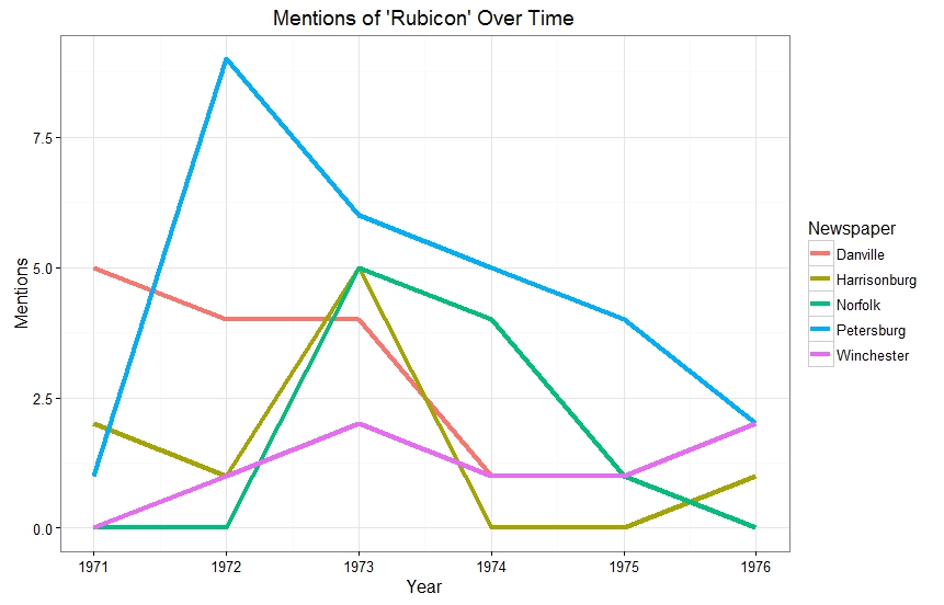
The Danville Register, The Harrisonburg Daily Record, The Norfolk Journal and Guide, The Petersburg Progress Index, The Winchester Star

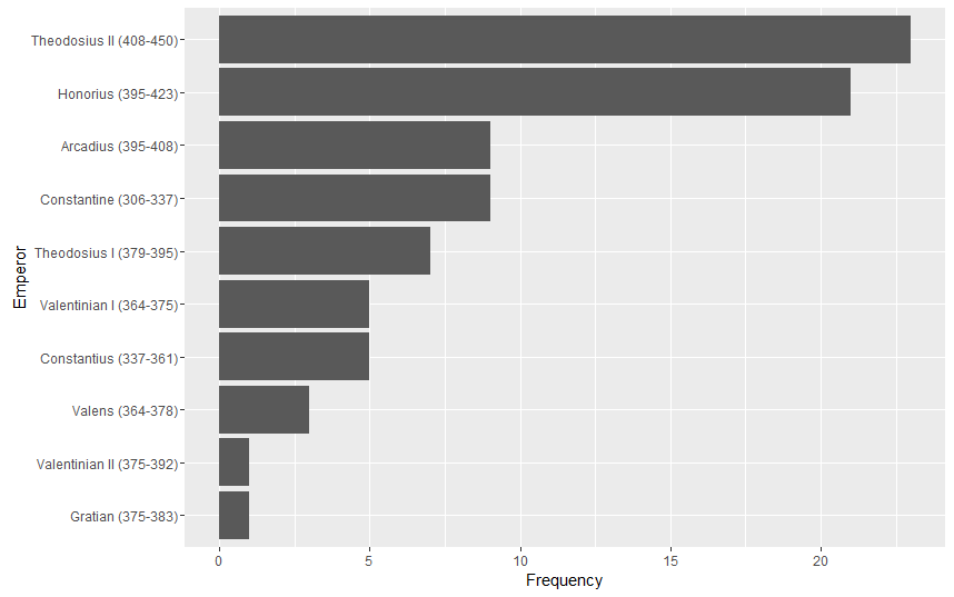
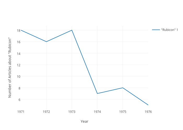
The graph above shows that mentions of Rubicon generally declined over time. This is probably dues to several factor: the decline in novelty, the slowing of intake at Rubicon, and shifting drug control priorities. It also reveals the relationship Rubicon had with Petersburg. Many of Rubicon’s admits were funneled to them through the Petersburg court system. Interestingly enough mentions in the two cities with the Rubicon facilities near there localities drop of in 1973. This is in line with larger statewide drug arrest trends that show a dip in arrests in 1973.

Most Characteristic Words in the Corpus

tf-idf-formula


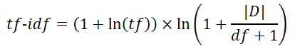
Using TF-IDF(term frequency-inverse document frequency) statistic to extract key terms from the four newspapers that wrote the most about Rubicon can provide a distant look at the semantic difference between newspapers. For more on TF-IDF see Kan Nashida’s blog.


tfidf


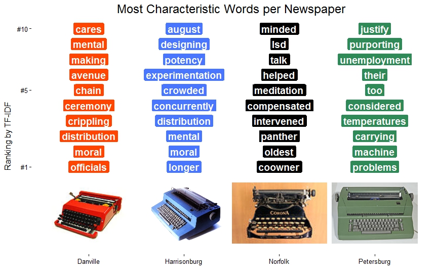
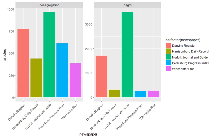
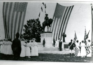
As can be seen TF-IDF produces some interesting results. The Danville newspaper uses words like “cares, “ceremony”, and “morals”, showing an interest in the positive impact of Rubicon. It also uses words like “chain”,”officials”, and “mental” which may reflect an interest in the organizational mechanics of Rubicon.  Similarly, Harrisonburg uses words like  “experimentation”, “crowded”, and, “designing” that imply and interest in how Rubicon was ran and maintained. The overlap of words between Harrisonburg and Danville may be due to proximity. The two cities were farther away from Rubicon then Norfolk and Petersburg and likely relied on the same AP reports. The Norfolk Journal and Guide is the only historically black newspaper in the corpus and discusses the black panthers more according to the TF-IDF metric. It is also the only newspaper that has a drug word(LSD) in its top ten of most characteristic words. Words like “mediated”, “helped”, and, “intervened” point to the expansion of Rubicon into the Norfolk area in 1973. Words in the Petersburg Progress Index reflect a similar closeness between Petersburg and Rubicon. “Unemployment”, “problems” and the disproportionately frequent use of “their” signify close economic and organizational ties.

Correlations

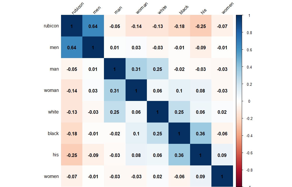
Correlation Matrices are another text-mining tool that can help shed light on Rubicon without a close reading. Correlations measure the strength of the relationship between variables. A correlation <0 indicates a negative relationship while a correlation>0 indicates a positive relationship.

rubicon-dem-corr


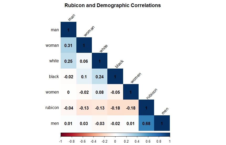
The matrix above shows a close correlation between the word “Rubicon” and the plural “men” across the whole corpus. On the other hand, it also shows a negative correlation between “Rubicon”, and the plural “women”. Surprisingly, race did not play a significant role in the coverage of Rubicon in the newspapers even though it appeared frequently throughout the press during this period.

race

rubicon-and-justice


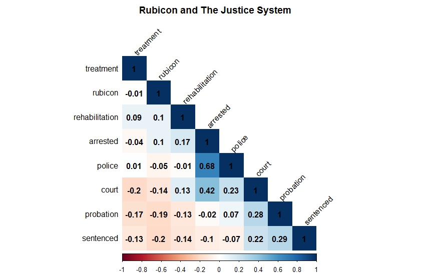
Rubicon’s relationship with the workings of the justice system is a bit more nuanced. Its important to remember that all of the newspapers mention Rubicon. The fact that Rubicon does not correlate highly with “rehabilitation” and “treatment” shows that Rubicon had reached a level of public notoriety that it no longer had to be described using these terms. Even so there is still a positive correlation between it and the words “arrested” and “court.”

kelly-and-menken


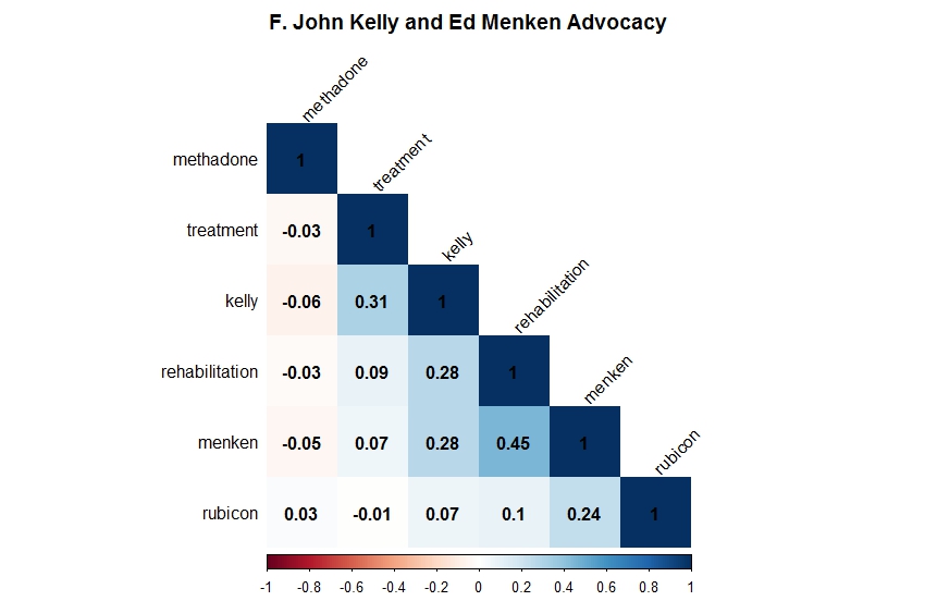
F. John Kelly, the director of the Governor’s Council on Narcotics and Drug Abuse Control, and Ed Menken the director of Rubicon had a sometimes contentious relationship in the press.  Menken frequently accused Kelly of taking a soft approach toward drug rehabilitation. The graphic above shows that Kelly correlates more highly with “treatment” but not “rehabilitation” than Menken. This could just be a matter of different word choices between the two after all Kelly is mentioned in 12 different articles while Menken is only mentioned in 6.

The positive correlation between Kelly and Menken denotes the level of dialog between the two. From the view of the frequent newspaper reader Kelly and Menken were locked in constant debate over rehabilitation resources and agendas. This constant pairing would have made Menken seem less like the Director of a private rehab and more like Kelly political equivalent. Another surprise from figure 6 is the lack of correlation between Kelly, Menken, and Rubicon with the word “methadone.”  Despite their advocacy for rehabilitation and treatment neither Kelly or Menken wanted to broach the controversial topic of methadone.

 Conclusion


correlation


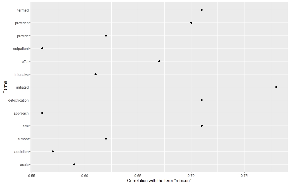
By analyzing the terms that correlate with Rubicon its institutional identity clearly exceeds that of its grassroots activist identity. Clinical terms like “detoxification”, “termed”, “outpatient”, “intensive”, “acute”, “provide”, and “offer” speak the business and medical side of the organization, and perhaps signify its movement toward a rehab ran by medical professionals rather than former addicts.  Coverage of Rubicon in the Virginia press neutralized the racial and activist components of the organization, thus helping to perpetuate the image of it as a state institution that both engaged in policy discussions and became a component of the justice system.

Code

library(stringr)
 library(corrplot)
 library(ggplot2)
 Convert Download articles into .txt and place in dataframe
 # folder with article PDFs
 dest <- "C:\\Users\\virgo\\Desktop\\Rubicon"
 # make a vector of PDF file names
 myfiles # convert each PDF file that is named in the vector into a text file
 # text file is created in the same directory as the PDFs
 # use pdftotxt.exe
 lapply(myfiles, function(i) system(paste('"C:\\Users\\Virgo\\Destop\\xpdf/bin64/pdftotext.exe"', paste0('"', i, '"')), wait = FALSE) )
 #create vector of txt file names
 rubiconfiles<-list.files(path = dest, pattern= "txt", full.names = TRUE)
 #turn into a list
 obj_list rubicon<-data.frame(obj_list)
 Clean up rubicon
 ##import rubicon.csv
 ##convert article text into lowercase and turn it into a string
 rubicon$Text<-tolower(rubicon$Text)
 rubicon.string ## split the string into words
 rubicon.string Word.list.df colnames(Word.list.df) ## remove blanks,lower, numbers
 Word.list.df Word.list.df$word<-tolower(Word.list.df[,1])
 Word.list.df ###create DTM
 target.list DTM.df ncol = length(target.list)))
 for (i in seq_along(target.list))
 {
 DTM.df[,i] }
 colnames(DTM.df) #nornalize DTM
 total.words DTM.matrix DTM.matrix DTM.norm.df #For Figure 2
 ###import rubicon mentions.csv and create line graph that shows mention of rubicon overtime
 ggplot(yy, aes(Year,Mentions))+geom_line(aes(colour=Newspaper), size=1.5)+labs(title="Mentions of 'Rubicon' Over Time") + xlab("Year") + ylab("Mentions") +theme_bw()
 For Correlations
 ##correlation
 short.list DTM.norm.mini.df #To get the correlation matrix
 cor.matrix.mini round(cor.matrix.mini, 2) ## rounds off at 2 places
 corrplot(cor.matrix.mini, method="shade",shade.col=NA,tl.col="black",tl.srt=45,addCoef.col="black",order="AOE", type="lower",title="Rubicon and Demographic Correlations",mar=c(0,0,2,0) )
 For Figure 8
 #word associations
 findAssocs(DTM, "rubicon", 0.57)
 #build dataframe for plotting
 toi <- "rubicon" # term of interest
 corlimit rubiconterms Terms = names(findAssocs(DTM, toi, corlimit)[[1]]))
 ggplot(rubiconterms, aes( y = Terms)) +geom_point(aes(x = corr), data = rubiconterms, size=2) +xlab(paste0("Correlation with the term ", "\"", toi, "\""))
 For Figure 3
 library(tm)
 library(RWeka)
 library(stringr)
 #import rubicon.csv and condense into articles by paper
 by.paper<-NULL
 for(paper in unique(rubicon$X4)){
 subset text row by.paper }
 # create corpus
 myReader corpus # pre-process text
 corpus corpus corpus corpus corpus # create term document matrix
 tdm<-TermDocumentMatrix(corpus)
 # remove sparse terms
 tdm. # save as a simple data frame
 count.all count.all$word write.csv(count.all, "C:\\Users\\virgo\\Desktop\\folder\\tdm.csv", row.names=FALSE)
 #normalize
 ## paste the text into one long string
 big.string ## split the string into words
 big.string ## get a dataframe of word frequency
 Word.list.df ## give the dataframe some nice names
 colnames(Word.list.df) ## remove blanks
 Word.list.df ## add \\b so the words are ready for regex searches
 target.list Word.list.df function(x) str_count(by.paper$text, x)
 count.matrix <-
 sapply(X = target.list, FUN = function(x) str_count(by.paper$text, x))
 ## lines below are clean up
 DTM.df colnames(DTM.df) DTM.matrix DTM.matrix DTM.norm.df paper.tfidf.df function(x) x*log(nrow(DTM.norm.df)/(sum(x!=0)+1))))
 rownames(paper.tfidf.df)<-c("Danville","Harrisonburg","Petersburg","Radford","Winchester","Norfolk")
 x<-6
 Tfidf.ten.df ## transpose for easier sorting
 Tfidf.ten.df ## add words
 Tfidf.ten.df$words ## sort and get top ten
 tfidf.ten tfidf.ten$words
 ###plot tfidf
 n p d h mycolors colnames(p)[1]<-"paper"
 colnames(p)[2]<-"word"
 ggplot(p, aes(paper, rank)) +
 geom_point(color="white") +
 geom_label(aes(label=p$word,fill=p$paper), color='white', fontface='bold', size=5) +
 scale_fill_manual(values = mycolors) +
 theme_classic() +
 theme(legend.position=1,plot.title = element_text(size=18), axis.title.y=element_text(margin=margin(0,10,0,0))) +
 labs(title="Most Characteristic Words per Newspaper") +
 xlab("") + ylab("Ranking by TF-IDF") +
 scale_y_continuous(limits=c(-4,10), breaks=c(1,6,10), labels=c("#1","#5", "#10")) +
 annotation_custom(Norfolk, xmin=.5, xmax=1.5, ymin=0, ymax=-4) +
 annotation_custom(Petersburg, xmin=1.5, xmax=2.5, ymin=0, ymax=-4) +
 annotation_custom(Danville, xmin=2.5, xmax=3.5, ymin=0, ymax=-4) +
 annotation_custom(Harrisonburg, xmin=3.5, xmax=4.5, ymin=0, ymax=-4)
 For Figure 5
 #import csv or race articles numbers
 p<-ggplot(race,aes(x=newspaper, y=articles,fill=as.factor(newspaper))) + geom_bar(stat="identity")+facet_wrap(~word, scales = "free")+theme(axis.text.x = element_text(angle = 45, hjust = 1))


The statistic results on map

The difference of percentage (provinces scale) between Manchu and Chinese version on map combines the line of the Coastal Exclusion Policy.
rplot04

The difference of percentage (cities scale) between Manchu and Chinese version on map combines the line of the Coastal Exclusion Policy.

rplot05

Coding is below.

##————————————————————————————————–##

rm(list=ls())
fileEncoding= “UTF-8”

## read file
setwd(“~/Desktop/003_PhD/016_Coursework/003_2016 Fall/003_HIST582A/003_Text”)
library(stringr)

## scan Chinese and Manchu texts
Chinese.vol.1.txt <- scan(“PDHF_Chinese_1.txt”, what = “chr”)
Chinese.vol.2.txt <- scan(“PDHF_Chinese_2.txt”, what = “chr”)
Chinese.vol.3.txt <- scan(“PDHF_Chinese_3.txt”, what = “chr”)
Manchu.vol.1.txt <- scan(“PDHF_Manchu_1.txt”, what = “chr”)
Manchu.vol.2.txt <- scan(“PDHF_Manchu_2.txt”, what = “chr”)
Manchu.vol.3.txt <- scan(“PDHF_Manchu_3.txt”, what = “chr”)

##————————————————————————————————–##
## [toponym counts] ##
## read table of place names in Chinese, Manchu, and English
Ch.place.names <- read.table(“Chinese_place_names.txt”, stringsAsFactors = FALSE)
Man.place.names <- read.table(“Manchu_place_names.txt”, sep=”\t”, stringsAsFactors = FALSE)
Eng.place.names <- read.table(“English_place_names.txt”, sep=”\t”, stringsAsFactors = FALSE)

## creating a new colname
Man.place.names$places <- tolower(Man.place.names$V1)
Ch.place.names$places <- tolower(Ch.place.names$V1)
Eng.place.names$places <- tolower(Eng.place.names$V1)
Ch.toponym <- unique(Ch.place.names$V1)
Man.toponym <- unique(Man.place.names$places)
Eng.toponym <- unique(Eng.place.names$V1)

## paste the full text
Manchu1 <- tolower(paste(Manchu.vol.1.txt, collapse = ” “))
Manchu2 <- tolower(paste(Manchu.vol.2.txt, collapse = ” “))
Manchu3 <- tolower(paste(Manchu.vol.3.txt, collapse = ” “))
Chinese1 <- paste(Chinese.vol.1.txt, collapse = “”)
Chinese2 <- paste(Chinese.vol.2.txt, collapse = “”)
Chinese3 <- paste(Chinese.vol.3.txt, collapse = “”)

## make the full Chinese text as a dataframe
Ch.Texts.df <- rbind.data.frame(Chinese1, Chinese2, Chinese3, stringsAsFactors = FALSE)
Chinese_all <- paste(Ch.Texts.df, collapse =””)
Ch.Texts.df <- rbind.data.frame(Chinese1, Chinese2, Chinese3, Chinese_all, stringsAsFactors = FALSE)

## rename the colname
colnames(Ch.Texts.df) <- “texts”

Ch.Text.metrics <- data.frame(t(data.frame(lapply(Ch.toponym, FUN=function(x) str_count(Ch.Texts.df$texts, x)))))

## put the place as one colname
Ch.Text.metrics$places <- Ch.toponym

## make three colnames sequently
colnames(Ch.Text.metrics)[c(1:4)] <- c(“Chinese1”, “Chinese2”, “Chinese3”, “Chinese_all”)

## the same process of Chinese in the Manchu version
Man.Texts.df <- rbind.data.frame(Manchu1, Manchu2, Manchu3, stringsAsFactors = FALSE)
Manchu_all <- tolower(paste(Man.Texts.df, collapse = ” “))
Man.Texts.df <- rbind.data.frame(Manchu1, Manchu2, Manchu3, Manchu_all, stringsAsFactors = FALSE)
colnames(Man.Texts.df) <- “texts”

Man.Text.metrics <- data.frame(t(data.frame(lapply(Man.toponym, FUN=function(x) str_count(Man.Texts.df$texts, x)))))

Man.Text.metrics$places <- Man.toponym
colnames(Man.Text.metrics)[c(1:4)] <- c(“Manchu1”, “Manchu2”, “Manchu3”, “Manchu_all”)

## combine Chinese and Manchu dataframe together
Combined.df <- cbind.data.frame(Ch.Text.metrics, Man.Text.metrics)
Combined.df$Chinese1.perc <- Combined.df$Chinese1/sum(Combined.df$Chinese1)*100
Combined.df$Chinese2.perc <- Combined.df$Chinese2/sum(Combined.df$Chinese2)*100
Combined.df$Chinese3.perc <- Combined.df$Chinese3/sum(Combined.df$Chinese3)*100
Combined.df$Chinese_all.perc <- Combined.df$Chinese_all/sum(Combined.df$Chinese_all)*100
Combined.df$Manchu1.perc <- Combined.df$Manchu1/sum(Combined.df$Manchu1)*100
Combined.df$Manchu2.perc <- Combined.df$Manchu2/sum(Combined.df$Manchu2)*100
Combined.df$Manchu3.perc <- Combined.df$Manchu3/sum(Combined.df$Manchu3)*100
Combined.df$Manchu_all.perc<- Combined.df$Manchu_all/sum(Combined.df$Manchu_all)*100

## show the result
Combined.df$toponym <- paste(Combined.df[,10], Combined.df[,5], Eng.place.names$places, sep=” “)
Combined.df$toponym

##————————————————————————————————–##
## [Coastal exclusion policy] ##
library(ggmap)
chinastate.map<-get_map(location=”china”, zoom=10, maptype=”satellite”)

cities.cep<- c(“廣西壯族自治區欽州市”, “廣西壯族自治區北海市合浦縣”, “合浦县石城村”, “廣東省湛江市遂溪县乾留”,
“湛江市雷州市海康港”, “湛江市雷州市扶茂”, “廣東省湛江市徐聞縣”, “廣東省湛江市徐聞縣海安鎮”,
“廣東省湛江市雷州市深田村”, “廣東省湛江市雷州市”, “廣東省湛江市遂溪縣”, “廣東省湛江市遂溪縣長坡墩”,
“廣東省湛江市吴川市博茂”, “廣東省湛江市吳川市”, “廣東省茂名市電白區”,
“廣東省陽江市陽西縣雙魚村”, “廣東省陽江市”, “江門市恩平市”, “廣東省江門市開平市”, “新會區將軍山旅遊區”,
“廣東省江門市新會區崖門鎮”, “廣東省江門市新會區”, “新會區觀音山”, “佛山市順德區”, “中山市三角鎮”,
“中山市馬鞍村”, “南沙区小虎山”, “深圳市寶安區西鄉”, “深圳市大鵬所城”, “海丰县琵琶”, “廣東省汕尾市海豐縣”,
“揭陽市惠來縣”, “揭陽市惠來縣靖海鎮”, “广东省汕头市潮南区古埕”, “廣東省汕頭市潮陽區”,
“揭陽市揭東區鄒堂”, “廣東省揭陽市”, “廣東省潮州市”, “潮州市饒平縣”, “福建省漳州市詔安縣分水關”,
“福建省漳州市詔安縣”, “漳州市云霄县油甘公”, “漳州市漳浦縣”, “漳州市漳浦縣橫口圩”, “漳州市龙海市洪礁寨”,
“漳州市龍海市海澄鎮”, “福建省漳州市龍文區江東橋”, “廈門市同安區蓮花村”, “廈門市同安區”, “廈門市翔安區小盈嶺”,
“福建省泉州市南安市大盈”, “福建省晉江”, “福建省泉州市南安市”, “泉州市洛江区洛陽橋”,
“泉州市惠安县石任”, “泉州市泉港区九峰山”, “莆田市荔城區壺公山”, “莆田市涵江區江口鎮”, “福清市高嶺村”,
“福州市福清市”, “長樂市岐陽村”, “馬尾區閩安村”, “福州市連江縣”, “連江縣浦口鎮”, “蕉城區白鶴嶺”,
“福建省寧德市”, “福安市洋尾”, “福安市小留村”, “寧德市福安市”, “福鼎市沙埕鎮”)
geo.cities.cep <- geocode(cities.cep)
geo.cities.cep.df<- data.frame(geo.cities.cep)

ggmap(chinastate.map) + geom_point(data=geo.cities.cep, aes(x=lon, y=lat))+ xlim(c(108, 122)) +ylim(c(20,28))

##————————————————————————————————–##
## [map] ##
library(ggmap)
china.map<-get_map(location=”China”, zoom=10, maptype=”satellite”)

cities<- c(“福建省泉州南安市安平橋”, “福建省廈門市同安區丙洲”, “湖南省長沙市”, “廣東省潮州市”,
“中國福建省泉州市惠安縣崇武鎮”, “中國福建省三明市永安市大漳山”, “福建福州市連江縣定海古城”,
“印尼雅加達”, “福建省寧德市霞浦縣烽火島”, “中國福建省”, “福建省福州市”, “福建省福州市長樂市新塘”,
“江蘇省揚州市邗江區瓜洲鎮”, “中國廣東省”, “中國貴州省”, “福建省漳州市龍海市海澄鎮”,
“福建省福州市平潭縣海壇島”, “福建省福州市台江區河口新村”, “中國湖北省”, “廣東省惠州市”,
“江蘇省南京市”, “廣東省汕尾市陸豐市碣石鎮”, “中國江蘇省”, “金門縣”, “廣東省汕頭市濠江區馬滘”,
“福建省莆田市秀嶼區湄洲大道湄洲島”, “福建省福州市馬尾區閩安村”, “廣東省汕頭市南澳縣”,
“浙江省寧波市”, “普列莫爾斯基區海參崴”, “廣東省汕頭市龍湖區鷗汀”, “臺灣省澎湖”,
“福建省莆田市秀嶼區平海鎮”, “浙江省溫州市平陽縣”, “福建省泉州市”, “浙江省紹興市”,
“福建福州市平潭縣石牌洋”, “福建省泉州石井鎮”, “福建省泉州市惠安縣獺窟島”, “浙江省台州市”,
“臺灣台南”, “福建省龍岩市長汀縣汀州”, “福建省廈門市同安區”, “福建省漳州市東山縣”,
“福建省泉州市惠安縣”, “福建省泉州市晉江市圍頭村”, “浙江省溫州市”, “福建省漳州市龍海市浯嶼”,
“福建省廈門市翔安區斗門”, “福建省廈門市”, “福建省莆田市”, “福建省廈門市集美區潯尾”,
“福建省泉州市石獅市永寧鎮”, “湖南岳陽縣”, “福建省漳州市雲霄縣”, “福建省漳州市”,
“中國浙江省”, “江蘇省鎮江市”, “浙江省舟山市”, “福建省泉州石獅市”)

geo.cities <- geocode(cities)
geo.cities.df<- data.frame(geo.cities)

map.df <- cbind.data.frame(Combined.df, geo.cities.df)

library(maps)
library(mapdata)
library(ggplot2)
world.map<- borders(database=”world”)
ggplot()+ world.map+ coord_quickmap()

world.map<- borders(database=”world”, colour=”gray20″, fill=”gray60″)
ggplot() + world.map +
coord_map(projection = “gilbert”, xlim =c(100,140), ylim=c(-20,50)) +
xlab(“”) + ylab(“”)+ ggtitle(“Percentage difference map”)
##————————————————————————————————–##
## [The new try] ##
## mixed provinces and cities ##
## volume 1 ##
Combined.df$perc1.diff <- (Combined.df$Chinese1.perc – Combined.df$Manchu1.perc)
Combined.df$perc2.diff <- (Combined.df$Chinese2.perc – Combined.df$Manchu2.perc)
Combined.df$perc3.diff <- (Combined.df$Chinese3.perc – Combined.df$Manchu3.perc)
map.df <- cbind.data.frame(Combined.df, geo.cities.df)
map.df$type1 <- ifelse(map.df$perc1.diff>0, “Chinese”, “Manchu”)
map.df$type1 <- ifelse(map.df$perc1.diff == 0, NA, map.df$type1)
map.df$type2 <- ifelse(map.df$perc2.diff>0, “Chinese”, “Manchu”)
map.df$type2 <- ifelse(map.df$perc2.diff == 0, NA, map.df$type2)
map.df$type3 <- ifelse(map.df$perc3.diff>0, “Chinese”, “Manchu”)
map.df$type3 <- ifelse(map.df$perc3.diff == 0, NA, map.df$type3)
map.df$scale <- c(“city”, “city”, “city”, “city”, “city”, “city”, “city”, “province”, “city”,”province”, “city”, “city”, “city”,
“province”, “province”, “city”, “city”, “city”, “province”, “city”, “city”, “city”, “province”, “city”, “city”,
“city”, “city”, “city”, “city”, “city”, “city”, “city”, “city”, “city”, “city”, “city”, “city”, “city”, “city”,
“city”, “city”, “city”, “province”, “city”, “city”, “city”)

## only province in Manchu and Chinese##
## volume 1 ##
vol1bp<- ggplot() + world.map + geom_point(data = subset(map.df, scale== “province”), aes(x = lon, y = lat, color=type1, shape = scale, size=abs(perc1.diff))) +
guides(size = FALSE) +
geom_path(data = geo.cities.cep.df, aes(x = lon, y = lat, color = “Coastal Exclusion Policy”))+
coord_map(projection = “stereographic”, xlim = c(112, 123), ylim = c(21,34)) + ylab(“”) + xlab(“”) +
ggtitle(“Provinces in Volume 1”)

## volume 2 ##
vol2bp<- ggplot() + world.map + geom_point(data = subset(map.df, scale == “province”), aes(x = lon, y = lat, color=type2, shape = scale, size=abs(perc2.diff))) +
guides(size = FALSE) +
geom_path(data = geo.cities.cep.df, aes(x = lon, y = lat, color = “Coastal Exclusion Policy”))+
coord_map(projection = “stereographic”, xlim = c(112, 123), ylim = c(21,34)) + ylab(“”) + xlab(“”) +
ggtitle(“Provinces in Volume 2”)

## volume 3 ##
vol3bp<- ggplot() + world.map + geom_point(data = subset(map.df, scale == “province”), aes(x = lon, y = lat, color=type3, shape = scale, size=abs(perc3.diff))) +
guides(size = FALSE) +
geom_path(data = geo.cities.cep.df, aes(x = lon, y = lat, color = “Coastal Exclusion Policy”))+
coord_map(projection = “stereographic”, xlim = c(112, 123), ylim = c(21,34)) + ylab(“”) + xlab(“”) +
ggtitle(“Provinces in Volume 3”)

##only cities in Manchu and Chinese##
## volume 1##
vol1bc<- ggplot() + world.map + geom_point(data = subset(map.df, scale== “city”), aes(x = lon, y = lat, color=type1, shape = scale, size=abs(perc1.diff))) +
guides(size = FALSE) +
geom_path(data = geo.cities.cep.df, aes(x = lon, y = lat, color = “Coastal Exclusion Policy”))+
coord_map(projection = “stereographic”, xlim = c(112, 123), ylim = c(21,34)) + ylab(“”) + xlab(“”) +
ggtitle(“Cities in Volume 1”)

## volume 2 ##
vol2bc<- ggplot() + world.map + geom_point(data = subset(map.df, scale== “city”), aes(x = lon, y = lat, color=type2, shape = scale, size=abs(perc2.diff))) +
guides(size = FALSE) +
geom_path(data = geo.cities.cep.df, aes(x = lon, y = lat, color = “Coastal Exclusion Policy”))+
coord_map(projection = “stereographic”, xlim = c(112, 123), ylim = c(21,34)) + ylab(“”) + xlab(“”) +
ggtitle(“Cities in Volume 2”)

##volume 3 ##
vol3bc<- ggplot() + world.map + geom_point(data = subset(map.df, scale== “city”), aes(x = lon, y = lat, color=type3, size=abs(perc3.diff))) +
guides(size = FALSE) +
geom_path(data = geo.cities.cep.df, aes(x = lon, y = lat, color = “Coastal Exclusion Policy”))+
coord_map(projection = “stereographic”, xlim = c(112, 123), ylim = c(21,34)) + ylab(“”) + xlab(“”) +
ggtitle(“Cities in Volume 1”)
## this function is from http://kanchengzxdfgcv.blogspot.tw/2016/11/r-ggplot2.html##
multiplot <- function(…, plotlist=NULL, file, cols=1, layout=NULL) {
library(grid)
plots <- c(list(…), plotlist)
numPlots = length(plots)
if (is.null(layout)) {
layout <- matrix(seq(1, cols * ceiling(numPlots/cols)),
ncol = cols, nrow = ceiling(numPlots/cols))
}

if (numPlots==1) {
print(plots[[1]])

} else {
grid.newpage()
pushViewport(viewport(layout = grid.layout(nrow(layout), ncol(layout))))
for (i in 1:numPlots) {
matchidx <- as.data.frame(which(layout == i, arr.ind = TRUE))

print(plots[[i]], vp = viewport(layout.pos.row = matchidx$row,
layout.pos.col = matchidx$col))
}
}
}
## provinces in both##
multiplot(vol1bp, vol2bp, vol3bp, cols= 1)

## cities in both##
multiplot(vol1bc, vol2bc, vol3bc, cols =1)

The Search for Modernity and Tradition in Fifteen Novels of Natsume Soseki

A Short Introduction of Natsume Soseki

1000_yen_natsume_soseki
Soseki’s Portrait on the old version of Japanese 1000 yen note

Natsume Soseki, born in 1867, the year before the Meiji Restoration, was a Japanese author whose works characterized the perplexity of Japanese during the era of rapid westernization. He loved Chinese literature, but studying English was a fashion at his time. Therefore, he became a scholar in English literature. The Japanese government sent him to study in England from 1901 to 1903, but this became his most unpleasant years. Soseki became mad in London, and started to question the idea of modernity. He was aware of the superficiality of Japanese westernization and aimless imitation of the west. In his works, he mainly focused on the pain and solitude that modernity brought to Japanese. Between 1905 and 1916, he wrote fifteen novels, including one unfinished. In 1907, Soseki rejected his professorship and started to work for Asahi newspaper, where most of his works were published. In 1916, he died of stomach ulcer.

Update on Historiographical Research

natsume-author-1

This is an update on last post. Natsume Soseki is commonly referred by his given name (or rather pen name), Soseki, so searching for “Soseki” in DfR of JSTOR collections is more accurate.

Text Mining of Soseki’s Novels

The central question that I am asking is what issues on modernity and tradition did Soseki write about and was Soseki more inclined to the traditional side or modern side.

The Japanese tokenizer MeCab with IPA dictionary takes in a txt file and produces a dataframe like the following graph. Term column is the word. Info1 is part of speech. Info2 is more information on part of speech.

rmecab
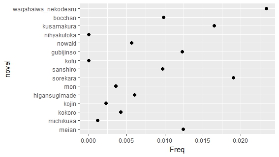
I processed the txt files with the same code I did a month ago, taking out pronunciation guide and style annotations. Then, I used dataframes generated by MeCab to calculate the term frequency in percentage and tf-idf. For all the graphs, the novels names on the axes are in chronological order

freq-gun
Total frequency in percentage of words that contain character 軍 (military) in each novel
freq-sen
Total frequency in percentage of words that contain character 戦 (war) in each novel

First, I focused on term frequency of some keywords. In last post I mentioned that English scholars were interested in discussion wars in studies of Japanese literature. This interests are not unjustified, since most of Soseki’s works mentioned words related to military and war. Meiji Japan was also a time of military victories, like Sino-Japanese War (1894-95) and Russo-Japanese War (1904-05). These were directly related to the westernization of Japan.

freq-ai
Total frequency in percentage of words that contain character 愛 (love) in each novel

Nevertheless, the word related to war was not that common compared to words related to love or death. In some of the works, Soseki showed his idea on love and solitude in modern world and how marriage in the new era should be different from old time. Maybe scholars should pay more attention to these issues.

For the other question, how did Soseki place himself in modernity and tradition. Although some famous critic, like Eto Jun thinks that Soseki stands on the side of tradition, especially in his last several works, more scholars argue that Soseki stands on side of modernity. Soseki was aware of the pain brought by westernization to Japanese, but he did not deny it. In some of his essays, he justified Japanese colonization of Manchuria and Korea by commenting that this was an inevitable result of a modernizing Japan.

The following figure presents frequency of four words, restoration (維新), enlightenment (開化), modernity (現代) and independent (独立), directly related to modernity and Meiji Restoration, in his novels. All of the novels used at least one of the four words.
gendai-freq
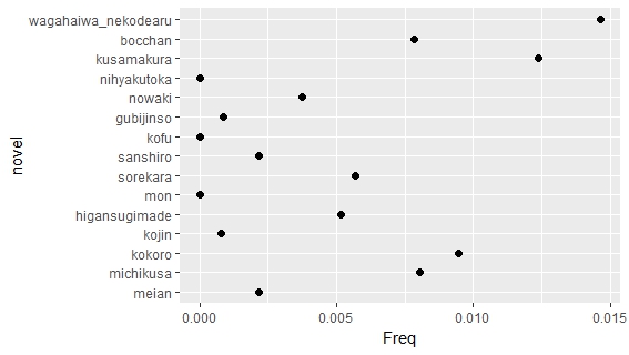
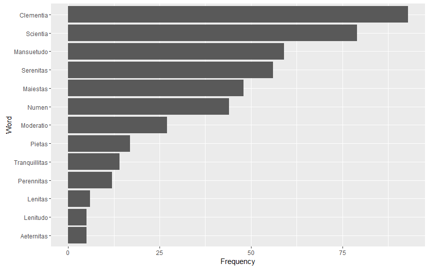
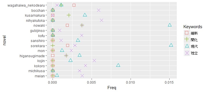
The following graph is a comparison between the frequencies the word modernity (現代) and antiquity (古代).Soseki used a lot more modernity than antiquity.  I wanted to find the frequency of tradition (伝統) or national learning (国学), but it turned out that Soseki never used these words.

gvk
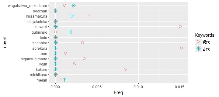
It might be the case that words like tradition or national learning emphasize superiority of Japanese culture, so Soseki avoided using them. His was disgusted by shallow nationalist movement of his classmates when he was young. By contrast the word Chinese study appeared several time in his novels.
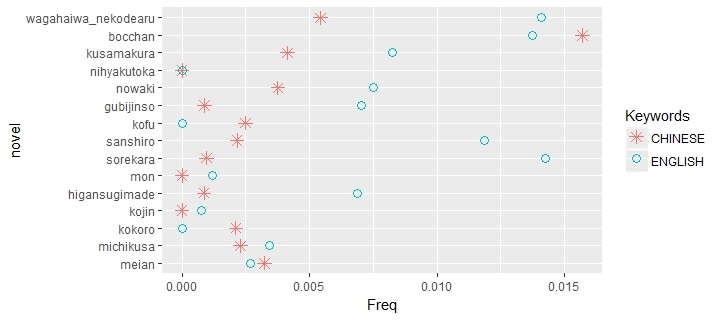
Another way of looking at the question is to search for the words related to Chinese and English. For Soseki, Chinese is the more traditional culture and English is more modern, while the westernizing Japan is somewhere between modernity and tradition. Related words to Chinese include Qing Empire (清国), Japan-Qing (日清), China (中国), Chinese book (漢籍), Chinese land (漢土) and Chinese poetry (漢詩); related words to English include the UK (イギリス or 英国), English (英語 or 英文), Anglo-Japanese (英和) and English translation (英訳)

This graph is not as extreme as last one. Although words related to English is still more important, words related to Chinese appear a lot.

eng-chnTf-idf

tf-idf-formula

The above equation is what I used for tf-idf. Both term frequency and document frequency are normalized.

Some of the novels are more interesting than other. Kokoro (The Hearts) is one of Soseki’s most beloved novel. The following graph is the top 5 words by tf-idf for each novel. Kokoro has the lowest tf-idf index, because it does not use many uncommon word. In other novels, characters has names, so the names have high tf-idf index. However, Soseki is reluctant to give characters names in Kokoro, so the most distinctive word is Zoshigaya (雑司ヶ谷), which is a place name in Tokyo.

Edwin McClellan, who introduced Soseki to western audience and translated two of Soseki’s novels, comments that Soseki wrote Kokoro as an “allegory of sorts”. Isolation and pain of Sensei, the protagonist in Volumn 3 of Kokoro, could be troubles to any Meiji intellectuals. The work is not only stylistically simple as noted by McClellan, but also lexically simple as shown in following graphs.

all-novel-tf-idf-top5
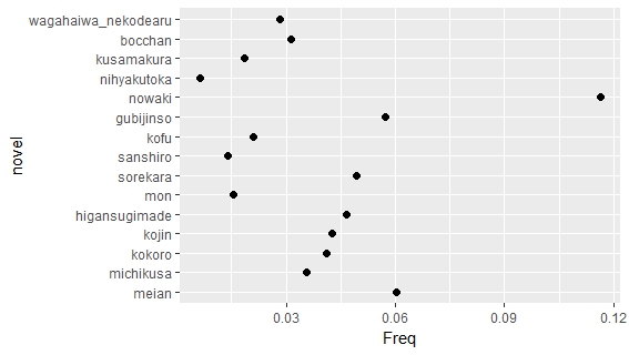
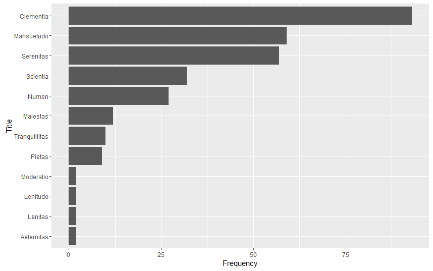
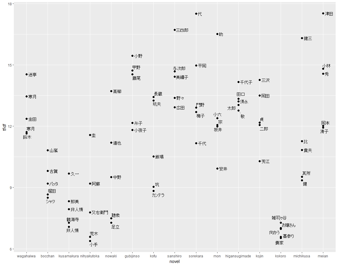
A violin graph of top 20 words by tf-idf also shows that Kokoro tends to use common word.
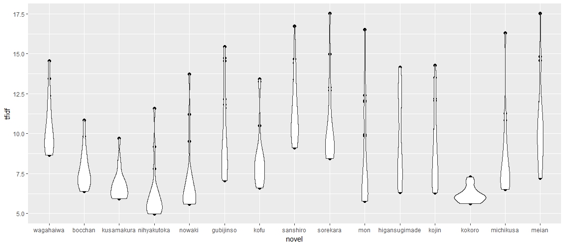
violin-tf-idf-top20Code

### Text Processing code is in the post about Dazai Osamu

### Make frequency tables with RMeCab

Sys.setlocale(“LC_ALL”, “Japanese”) ### Windows users may want to use this to avoid encoding problems

library(RMeCab) ### Japanese Tokenizer

na.zzz <- RMeCabFreq(“D:/Google Drive/JPN_LIT/Natsume/zzz.txt”)
na.zzz.reduced <- na.zzz[which(na.zzz$Info1 != “記号”),] ###Take out punctuations

files.cle.dir<- list.files(“D:/Google Drive/JPN_LIT/Natsume/cleaned”)

for (n.i in 1:length(files.cle.dir)){
assign(paste0(“n.”, files.cle.dir[n.i]), RMeCabFreq(paste0(“D:/Google Drive/JPN_LIT/Natsume/cleaned/”,files.cle.dir[n.i]))[which(RMeCabFreq(paste0(“D:/Google Drive/JPN_LIT/Natsume/cleaned/”,files.cle.dir[n.i]))$Info1 != “記号”),])
}

###A sample code of combining frequency table of a novel to the frequency table of the corpus of fifteen novels.

z <- 1
y <- 1
while (z <= length(na.zzz.reduced$Term)){
if(n.bocchan.txt$Term[y] == na.zzz.reduced$Term[z] & n.bocchan.txt$Info1[y] == na.zzz.reduced$Info1[z] & n.bocchan.txt$Info2[y] == na.zzz.reduced$Info2[z]){
na.zzz.reduced$bocchan[z] <- n.bocchan.txt$Freq[y]
y <- y + 1
}
z <- z + 1
}

### na.zzz.reduced is the final frequency dataframe with every novel

### Tf-idf

n.TMD <- na.zzz.reduced[,4:19]
n.TMD$Dfreq <- apply(n.TMD, 1, function(x) length(which(x != 0)))
n.TMD$Dfnorm <- log(15/n.TMD$Dfreq +1)

n.TFIDF.df <- data.frame(t(apply(n.TMD[,2:16], 1, function(x) log(x)+1)))
n.TFIDF.df <- n.TFIDF.df*n.TMD$Dfnorm
n.TFIDF.df[n.TFIDF.df == -Inf] <- 0

Final.TFIDF.df <- cbind(na.zzz.reduced[,1:3],n.TFIDF.df)

##### Make another table of Final percentage

n.PERC.df<- data.frame(apply(n.TMD[,1:16], 2,function(x) x/sum(x)*100))
Final.PERC.df <- cbind(na.zzz.reduced[,1:3],n.PERC.df)


###Make a dataframe of top 20 and top 5 tfidf for each novel and change the name of wagahaiwa_nekodearu since it is too long
all.TFIDF20 <- data.frame(Term = NA,tfidf = NA, novel = NA)
for (col.i in 4:18){
all.TFIDF20 <- rbindlist(list(all.TFIDF20, cbind(Final.TFIDF.df[order(-Final.TFIDF.df[,col.i]),][1:20,][,c(1,col.i)],colnames(Final.TFIDF.df)[col.i])))
}
all.TFIDF20 <- all.TFIDF20[-1,]
all.TFIDF20$novel <- as.character(all.TFIDF20$novel)
all.TFIDF20[all.TFIDF20 == “wagahaiwa_nekodearu”] <- “wagahaiwa”

### Top5 tf-idf

all.TFIDF5 <- data.frame(Term = NA,tfidf = NA, novel = NA)
for (col.i in 4:18){
all.TFIDF5 <- rbindlist(list(all.TFIDF5, cbind(Final.TFIDF.df[order(-Final.TFIDF.df[,col.i]),][1:5,][,c(1,col.i)],as.character(colnames(Final.TFIDF.df)[col.i]))))
}
all.TFIDF5 <- all.TFIDF5[-1,]
all.TFIDF5$novel <- as.character(all.TFIDF5$novel)

### Violin Graph

ggplot(all.TFIDF20, aes(x = novel, y = tfidf))+
geom_point(size = 2) +
scale_x_discrete(limits=c(“wagahaiwa”,”bocchan”,”kusamakura”,”nihyakutoka”,”nowaki”,”gubijinso”,”kofu”,”sanshiro”,”sorekara”,”mon”,”higansugimade”,”kojin”,”kokoro”,”michikusa”,”meian”)) +
geom_violin()

### Top 5 tf-idf with term shown

library(ggrepel) ### An extension to ggplot2 to avoid overlap of terms in graph

ggplot(all.TFIDF5, aes(x = novel, y = tfidf))+
geom_point(size = 2) +
scale_x_discrete(limits=c(“wagahaiwa”,”bocchan”,”kusamakura”,”nihyakutoka”,”nowaki”,”gubijinso”,”kofu”,”sanshiro”,”sorekara”,”mon”,”higansugimade”,”kojin”,”kokoro”,”michikusa”,”meian”)) +
geom_text_repel(aes(label=Term), size =4, segment.color = ‘grey60’,nudge_x =0.05)

### A sample graph of how I made the table for words related to Chinese and English. All other frequency graphs are similar (I admit that I used Mspaint to change some of the legend, because it is more convenient)
chn.all.PERC.df <- Final.PERC.df[which(Final.PERC.df$Term == “清国” |
Final.PERC.df$Term == “中国”|
Final.PERC.df$Term == “漢学”|
Final.PERC.df$Term ==”漢語”|
Final.PERC.df$Term ==”漢詩”|
Final.PERC.df$Term ==”漢籍”|
Final.PERC.df$Term ==”漢土”|
Final.PERC.df$Term ==”漢”|
Final.PERC.df$Term ==”漢人”),] ### I choose the terms based on search for three words, “清”, “漢” and “中国”.

eng.all.PERC.df <- Final.PERC.df[which(Final.PERC.df$Term == “イギリス” |
Final.PERC.df$Term == “英国”|
Final.PERC.df$Term == “英訳”|
Final.PERC.df$Term ==”英語”|
Final.PERC.df$Term ==”英文”|
Final.PERC.df$Term ==”英和”),]### The choice of vocabularies is similarly determined by the research intention
chn.eng.df <- data.frame(apply(chn.all.PERC.df[,5:19], 2, function(x) sum(x)))
chn.eng.df <- cbind(chn.eng.df, data.frame(apply(eng.all.PERC.df[,5:19], 2, function(x) sum(x))))

colnames(chn.eng.df) <- c(“CHINESE”, “ENGLISH”)

chn.eng.df$novel <- row.names(chn.eng.df)

ggplot(chn.eng.df, aes(x = novel))+
geom_point(aes(y=CHINESE, color = “CHINESE”), shape = 8, size =3) +
geom_point(aes(y=ENGLISH, color = “ENGLISH”), shape = 1, size =3) +
scale_x_discrete(limits=rev(c(“wagahaiwa_nekodearu”,”bocchan”,”kusamakura”,”nihyakutoka”,”nowaki”,”gubijinso”,”kofu”,”sanshiro”,”sorekara”,”mon”,”higansugimade”,”kojin”,”kokoro”,”michikusa”,”meian”))) +
labs(color=”Keywords”)+
ylab(“Freq”) +
coord_flip()

Imperial Titles in the Theodosian Code

Frequency of Imperial Titles in the Theodosian Code

titlesincth


Frequency of Those Words (not just as titles) in the Theodosian Code

nontitle


Frequency of Clementia as Imperial Title, by Reign

byreign


Code

#THEODOSIAN CODE

CTh.scan <- scan(“~/Education/Emory/Coursework/Digital Humanities Methods/Project/Theodosian Code Raw Text.txt”,
what=”character”, sep=”\n”)
CTh.df <- data.frame(CTh.scan, stringsAsFactors=FALSE)
CTh.df <- str_replace_all(string = CTh.df$CTh.scan, pattern = “[:punct:]”, replacement = “”)
CTh.df <- data.frame(CTh.df, stringsAsFactors = FALSE)
CTh.lines <- tolower(CTh.df[,1])
book.headings <- grep(“book”, CTh.lines)
start.lines <- book.headings + 1
end.lines <- book.headings[2:length(book.headings)] – 1
end.lines <- c(end.lines, length(CTh.lines))
CTh.df <- data.frame(“start” = start.lines, “end”=end.lines, “text”=NA)
i <- 1
for (i in 1:length(CTh.df$end))
{CTh.df$text[i] <- paste(CTh.lines[CTh.df$start[i]:CTh.df$end[i]], collapse = ” “)}

CTh.df$Book <- seq.int(nrow(CTh.df))

#String Extracts of Imperial Titles

str_extract_all(string = CTh.df$text, pattern = “.{0,80}nostra.{0,80}aeternita.{0,80}|.{0,80}aeternita.{0,80}nostra.{0,80}|.{0,80}mea.{0,80}aeternita.{0,80}|.{0,80}aeternita.{0,80}mea.{0,80}”) #AETERNITAS

str_extract_all(string = CTh.df$text, pattern = “.{0,80}nostra.{0,80}clementia.{0,80}|.{0,80}clementia.{0,80}nostra.{0,80}|.{0,80}mea.{0,80}clementia.{0,80}|.{0,80}clementia.{0,80}mea.{0,80}”) #CLEMENTIA

str_extract_all(string = CTh.df$text, pattern = “.{0,80}nostra.{0,80}lenita.{0,80}|.{0,80}lenita.{0,80}nostra.{0,80}|.{0,80}mea.{0,80}lenita.{0,80}|.{0,80}lenita.{0,80}mea.{0,80}”) #LENITAS

str_extract_all(string = CTh.df$text, pattern = “.{0,80}nostra.{0,80}lenitud.{0,80}|.{0,80}lenitud.{0,80}nostra.{0,80}|.{0,80}mea.{0,80}lenitud.{0,80}|.{0,80}lenitud.{0,80}mea.{0,80}”) #LENITUDO

str_extract_all(string = CTh.df$text, pattern = “.{0,80}nostra.{0,80}maiesta.{0,80}|.{0,80}maiesta.{0,80}nostra.{0,80}|.{0,80}mea.{0,80}maiesta.{0,80}|.{0,80}maiesta.{0,80}mea.{0,80}”) #MAIESTAS

str_extract_all(string = CTh.df$text, pattern = “.{0,80}nostra.{0,80}mansuetud.{0,80}|.{0,80}mansuetud.{0,80}nostra.{0,80}|.{0,80}mea.{0,80}mansuetud.{0,80}|.{0,80}mansuetud.{0,80}mea.{0,80}”) #MANSUETUDO

str_extract_all(string = CTh.df$text, pattern = “.{0,80}nostra.{0,80}moderatio.{0,80}|.{0,80}moderatio.{0,80}nostra.{0,80}|.{0,80}mea.{0,80}moderatio.{0,80}|.{0,80}moderatio.{0,80}mea.{0,80}”) #MODERATIO

str_extract_all(string = CTh.df$text, pattern = “.{0,80}nostrum.{0,80}numen.{0,80}|.{0,80}numen.{0,80}nostrum.{0,80}|.{0,80}nostr.{0,80}numin.{0,80}|.{0,80}numin.{0,80}nostr.{0,80}|.{0,80}meum.{0,80}numen.{0,80}|.{0,80}numen.{0,80}meum.{0,80}|.{0,80}me.{0,80}numin.{0,80}|.{0,80}numin.{0,80}me.{0,80}”) #NUMEN

str_extract_all(string = CTh.df$text, pattern = “.{0,80}nostra.{0,80}perennita.{0,80}|.{0,80}perennita.{0,80}nostra.{0,80}|.{0,80}mea.{0,80}perennita.{0,80}|.{0,80}perennita.{0,80}mea.{0,80}”) #PERENNITAS

str_extract_all(string = CTh.df$text, pattern = “.{0,80}nostra.{0,80}pieta.{0,80}|.{0,80}pieta.{0,80}nostra.{0,80}|.{0,80}mea.{0,80}pieta.{0,80}|.{0,80}pieta.{0,80}mea.{0,80}”) #PIETAS

str_extract_all(string = CTh.df$text, pattern = “.{0,80}nostra.{0,80}scientia.{0,80}|.{0,80}scientia.{0,80}nostra.{0,80}|.{0,80}mea.{0,80}scientia.{0,80}|.{0,80}scientia.{0,80}mea.{0,80}”) #SCIENTIA

str_extract_all(string = CTh.df$text, pattern = “.{0,80}nostra.{0,80}serenita.{0,80}|.{0,80}serenita.{0,80}nostra.{0,80}|.{0,80}mea.{0,80}serenita.{0,80}|.{0,80}serenita.{0,80}mea.{0,80}”) #SERENITAS

str_extract_all(string = CTh.df$text, pattern = “.{0,80}nostra.{0,80}tranquillita.{0,80}|.{0,80}tranquillita.{0,80}nostra.{0,80}|.{0,80}mea.{0,80}tranquillita.{0,80}|.{0,80}tranquillita.{0,80}mea.{0,80}”) #TRANQUILLITAS

#Imperial Title Sums

aeternitas <- 2
clementia <- 93
lenitas <- 2
lenitudo <- 2
maiestas <- 12
mansuetudo <- 59
moderatio <- 2
numen <- 27
perennitas <- 12
pietas <- 9
scientia <- 32
serenitas <- 57
tranquillitas <- 10

#Imperial Title Sum Graph

Frequency <- c(aeternitas, clementia, lenitas, lenitudo, maiestas, mansuetudo, moderatio, numen, perennitas, pietas, scientia, serenitas, tranquillitas)
Title <- c(“Aeternitas”, “Clementia”, “Lenitas”, “Lenitudo”, “Maiestas”, “Mansuetudo”, “Moderatio”, “Numen”, “Perennitas”, “Pietas”, “Scientia”, “Serenitas”, “Tranquillitas”)
sum.df <- cbind.data.frame(Title, Frequency)
sum.df$Title <- factor(sum.df$Title, levels = sum.df$Title[order(sum.df$Frequency)]) #Reorders dataframe based on Frequency

ggplot(data=sum.df, aes(x=Title, Frequency), y=Frequency) + geom_bar(stat = “identity”) + coord_flip() #Word Total Graph

#Non-Title Frequencies

aeternitas <- sum(str_count(CTh.df$text, “aeternita”), na.rm = TRUE)
clementia <- sum(str_count(CTh.df$text, “clementia”), na.rm = TRUE)
lenitas <- sum(str_count(CTh.df$text, “lenita”), na.rm = TRUE)
lenitudo <- sum(str_count(CTh.df$text, “lenitud”), na.rm = TRUE)
maiestas <- sum(str_count(CTh.df$text, “maiesta”), na.rm = TRUE)
mansuetudo <- sum(str_count(CTh.df$text, “mansuetud”), na.rm = TRUE)
moderatio <- sum(str_count(CTh.df$text, “moderatio”), na.rm = TRUE)
numen <- sum(str_count(CTh.df$text, “numen|numin”), na.rm = TRUE)
perennitas <- sum(str_count(CTh.df$text, “perennita”), na.rm = TRUE)
pietas <- sum(str_count(CTh.df$text, “pieta”), na.rm = TRUE)
scientia <- sum(str_count(CTh.df$text, “scientia”), na.rm = TRUE)
serenitas <- sum(str_count(CTh.df$text, “serenita”), na.rm = TRUE)
tranquillitas <- sum(str_count(CTh.df$text, “tranquillita”), na.rm = TRUE)

Frequency <- c(aeternitas, clementia, lenitas, lenitudo, maiestas, mansuetudo, moderatio, numen, perennitas, pietas, scientia, serenitas, tranquillitas)
Title <- c(“Aeternitas”, “Clementia”, “Lenitas”, “Lenitudo”, “Maiestas”, “Mansuetudo”, “Moderatio”, “Numen”, “Perennitas”, “Pietas”, “Scientia”, “Serenitas”, “Tranquillitas”)
sum.df <- cbind.data.frame(Title, Frequency)
sum.df$Title <- factor(sum.df$Title, levels = sum.df$Title[order(sum.df$Frequency)]) #Reorders dataframe based on Frequency

ggplot(data=sum.df, aes(x=Title, Frequency), y=Frequency) + geom_bar(stat = “identity”) + coord_flip() #Word Total Graph

#Title Frequency By Reign

constantine <- 9
constantius <- 5
valentinian1 <- 5
valens <- 3
gratian <- 1
valentinian2 <- 1
theodosius1 <- 7
honorius <- 21
arcadius <- 9
theodosius2 <- 23

Frequency <- c(constantine, constantius, valentinian1, valens, gratian, valentinian2, theodosius1, honorius, arcadius, theodosius2)
Title <- c(“Constantine (306-337)”, “Constantius (337-361)”, “Valentinian I (364-375)”, “Valens (364-378)”, “Gratian (375-383)”, “Valentinian II (375-392)”, “Theodosius I (379-395)”, “Honorius (395-423)”, “Arcadius (395-408)”, “Theodosius II (408-450)”)
sum.df <- cbind.data.frame(Title, Frequency)
sum.df$Title <- factor(sum.df$Title, levels = sum.df$Title[order(sum.df$Frequency)]) #Reorders dataframe based on Frequency

ggplot(data=sum.df, aes(x=Title, Frequency), y=Frequency) + geom_bar(stat = “identity”) + labs(x = “Emperor”) + coord_flip() #Word Total Graph

Rubicon Newspaper Corpus Visualizations

Rubicon and Demographics Correlation Matrix

democorr


Terms that Correlate Strongly With “Rubicon”

correlation


##correlation Matrix code. Start from normalized document term matrix
Library(corrplot)
short.list DTM.norm.mini.df #To get the correlation matrix
cor.matrix.mini round(cor.matrix.mini, 2) ## rounds off at 2 places
corrplot(cor.matrix.mini, method=”shade”,shade.col=NA,tl.col=”black”,tl.srt=45,addCoef.col=”black”,order=”FPC”)#word associations start from DTM
Library(tm)
Library(ggplot2)
findAssocs(DTM, “rubicon”, 0.57)
#build dataframe for plotting
toi <- “rubicon” # term of interest
corlimit rubiconterms Terms = names(findAssocs(DTM, toi, corlimit)[[1]]))
ggplot(rubiconterms, aes( y = Terms)) +geom_point(aes(x = corr), data = rubiconterms, size=2) +xlab(paste0(“Correlation with the term “, “\””, toi, “\””))


timeline1

Final Project/Post

A ‘Mecca of Patriotism’: The Commemorative Monuments of the Guilford Battle Ground Park and Shifting Views toward Historic Preservation

Greene Monument

Nathanael Greene Monument. Photo courtesy of the National Park Service.

Guilford Courthouse National Military Park is located in north-central North Carolina about six miles northwest of downtown Greensboro. The park encompasses about 220 acres, which protect the core of the largest, most hotly contested battle of the American Revolution’s climactic Southern Campaign. In 1887, under the direction of Judge David Schenck, the Guilford Battle Ground Company (GBGC) was chartered for the purpose of preserving and adorning the American Revolution battlefield at Guilford Courthouse in North Carolina. Motivated foremost by patriotism, the GBGC erected approximately 30 monuments and memorials between 1888 and 1917 at the Guilford Battle Ground Park, of which seven marked grave sites.  The history of commemoration at Guilford reflects the developing national commemorative movement that emerged in America in the late 1800s and continued through the early 1900s.

While the GBGC erected the majority of monuments at the battlefield, the War Department continued the tradition from 1917 through 1933 by adding five monuments at the newly established Guilford Courthouse National Military Park (GUCO NMP). Since the National Park Service (NPS) began managing GUCO NMP in 1933, it has removed six monuments from the battlefield and relocated others. In 2016, GUCO NMP gained a new monument sponsored by the reinstated Guilford Battle Ground Company with assistance from several British Regimental Associations to recognize the British Regiments associated with the battle. This monument was the first erected at Guilford in nearly 84 years, as well as the only one associated with the NPS’s management period.

Although the GBGC, the War Department, and the NPS have shared the same underlying goal of preserving the historic Guilford battlefield, each entity has taken its own approach to achieve this end. In my paper, I will examine how the creation and removal of monuments throughout the various periods at Guilford correlate with shifting cultural attitudes and ideas toward commemoration and historic preservation. I will use a combination of qualitative and quantitative methods to identify patterns in the monuments at Guilford—ranging from the individuals and groups who sponsored the monuments to the subjects they honored, their materials, artistic styles, and distinct placement in the landscape.

Monuments at Guilford Courthouse NMP

Above, a positive and negative bar graph showing trends in the erection and removal of monuments at Guilford Courthouse National Military Park across the decades in relation to its different periods of management under the Guilford Battle Ground Company, the War Department, and the National Park Service.

Ngram

Above, image from the Google Books Ngram Viewer showing how the words “monument” and “patriotism” have occurred throughout a corpus of American English books from 1880-2000. The peak and decline in use of this word in writing generally follows the overall trend of the erection and removal of monuments at Guilford and other sites across the country.

Late 1800s Late 1800s populaiton

Above, line graphs shows how the development of the Guilford Battle Ground Park paralleled the growth of the city of Greensboro.

In 1890, Schenck wrote:

“Now that Greensboro has the certain prospect of becoming a large city and extending northward towards the Battle Ground, it is easy to foresee that so interesting and beautiful a place as this, abounding in shade, and supplied with abundance of the purest water, must in the near future, become the park of the city, where its citizens can go for rest and recreation; and that summer cottages will be built up around it where the families of the city can escape the heat and dust and enjoy the fresh air of a delightful country resort.”[1]

[1] David Schenck, “To the Stockholders of the Guilford Battle Ground Company, Greensboro, NC, March 15, 1890,” in David Schenck Papers, 1849-1917, Folder 16: Volume 15: 1887-1900: Scan 36 (Southern Historical Collection, The Wilson Library, University of North Carolina at Chapel Hill).

1890s

Above, a map showing the concentrations of monuments commemorating the American Revolution erected in North Carolina in the 1890s. In this decade, the state gained 10 new monuments commemorating the American Revolution of which nine were erected at the Guilford Battle Ground Park.

*During the first decade of the 20th century, the state did not gain any monuments commemorating the American Revolution. While Guilford (and other sites) did gain monuments during this period, the subjects they commemorated bore other associations. For example, during this decade the Guilford Battle Ground Company erected monuments to commemorate Judge David Schenck, the company’s first president, and to Clio, the Muse of History, among others.

1910s

Above, a map showing the concentrations of monuments commemorating the American Revolution erected in North Carolina in the 1910s. In the decade, commemoration expanded to other areas across the state, such as near the cities of Raleigh and Fayetteville, and Wilmington. Of the 17 monuments erected across the state during this period to commemorate the American Revolution, over half were at the Guilford Battle Ground Park. Note that the map also shows one American Revolution monument erected near the border in Blacksburg, South Carolina where the battle of Kings Mountain occurred.

1920s

Above, map showing the concentrations of monuments commemorating the American Revolution erected in North Carolina in the 1920s.

1930s

Above, map showing the concentrations of monuments commemorating the American Revolution erected in North Carolina in the 1930s. At this point, the numbers across the state are dwindling.

1940s

Above, map showing the concentrations of monuments commemorating the American Revolution erected in North Carolina in the 1940s. There were no other Revolutionary War monuments erected in the state until July 2016 when Guilford gained its new Crown Forces monument.

The following bar graphs show patterns in the materials, styles, and subjects of the monuments.

MaterialsStyles

The vast majority of the monuments at Guilford were carved from granite due to its abundance in the area and accessibility from the Mount Airy Granite Quarry. While several of the monuments incorporated cast bronze sculptures, many others contained bronze tablets with quotations. In the latter half of the nineteenth century, the popularity of bronze eclipsed marble as a medium for sculpture due to the development of specialized foundries and the proliferation of trained labor and equipment. Much of the bronze work at Guilford can be traced to two foundries: the Bureau Brothers of Philadelphia, Pennsylvania, and W. H. Mullins, Manufacturer of Architectural Sheet Metal Work and Statuary, of Salem, Ohio.

Subjects

In addition to seeing Guilford as a “park of the city,” Schenck also saw the site as the state’s common burial ground for the American Revolution. Accordingly, the vast majority of monuments at Guilford honored “successful heroes and statesmen.” There were a few, however, commemorating historical female figures, as well as others that commemorated other events, such as the Battle of Kings Mountain. Thus, it is not surprising that a large percentage of monuments at Guilford do not have a direct association with the Battle of Guilford Courthouse.

Pie Chart

The GBGC-era reveals how historic preservation was characterized by attempts to keep certain memories alive through the creation of monuments  and memorials. During the NPS-era, cultural attitudes shifted away from the production of monuments as historic preservation focused more on “authenticity” and “integrity” of the site’s Revolutionary War period. More recently, the NPS has begun to recognize the significance of the site’s commemorative period. Today, Guilford presents a key preservation challenge for its managers, who must determine how to balance the site’s past with its present as its significance continues to fluctuate over time.

R Codes

#To create a bar graph showing the addition and removal of Monuments at Guilford across the decades
library(ggplot2)
dat <- read.table(text = “ Variable Decade Monuments
1 Added 1880s 3
2 Removed 1880s 0
3 Added 1890s 10
4 Removed 1890s 0
5 Added 1900s 11
6 Removed 1900s 0
7 Added 1910s 4
8 Removed 1910s 0
9 Added 1920s 3
10 Removed 1920s 0
11 Added 1930s 3
12 Removed 1930s -4
13 Added 1940s 0
14 Removed 1940s 0
15 Added 1950s 0
16 Removed 1950s 0
17 Added 1960s 0
18 Removed 1960s -1
19 Added 1970s 0
20 Removed 1970s -1
21 Added 1980s 0
22 Removed 1980s 0
23 Added 1990s 0
24 Removed 1990s 0
25 Added 2000s 0
26 Removed 2000s 0
27 Added 2010s 1
28 Removed 2010s 0”,header = TRUE,sep = “”,row.names = 1)
dat1 <- subset(dat,Monuments >= 0)
dat2 <- subset(dat,Monuments < 0)

ggplot() +
geom_bar(data = dat1, aes(x=Decade, y=Monuments, fill=Variable),stat = “identity”) +
geom_bar(data = dat2, aes(x=Decade, y=Monuments, fill=Variable),stat = “identity”) +
geom_bar(stat = “identity”, color = “black”) +
scale_fill_manual(values =c(“#66cc99”, “#ff6666”)) +
guides(fill = guide_legend(override.aes = list(colour = NULL))) +
guides(colour = FALSE) +
ggtitle(“Monuments at Guilford Courthouse National Military Park”) +labs(x=”Decade”, y=”Number”) +
geom_hline(yintercept=0)

#To create a map of North Carolina showing the distribution of American Revolution monuments in the 1890s **I applied the same code to create other maps, but with different coordinates and sizes for the points. I had difficulty creating annotations in R so I used Adobe Illustrator.

library(ggmap)
myLocation <- c(-84.917575, 33.954619, -75.002153, 36.679869) #creates a map of North Carolina based on bottom left and top right coordinates
myMap <- get_map(location=myLocation,
source=”google”, maptype = “terrain”, crop=FALSE, zoom = 7) #defines the source and type of the map, as well as its zoom
ggmap(myMap)+
geom_point(aes(x = -80.842286, y = 35.222339), colour = “red”, alpha = .5, size = 4)+
geom_point(aes(x = -79.798653, y = 36.046642), colour = “red”, alpha = .5, size = 6) #defines the points on the map and their sizes

#To create a line graph showing the number of monuments erected at Guilford per decade in the late 1800s
monuments <- c(0, 3, 10, 11) #creates the point values for the line
g_range <- range(0, monuments) #creates the range for the y-axis
plot(monuments, type=”o”, col=”green”, ylim=g_range,
axes=FALSE, ann=FALSE) #plots the green line
axis(1, at=1:4, lab=c(“1870s”,”1880s”, “1890s”, “1900s”)) #adjusts the labels on the x-axis
axis(2, las=1, at=1*0:g_range[2]) #adjusts the tick marks on the y-axis
title(main=”Guilford Monuments Erected in the Late 19th Century”, col.main=”black”, font.main=4) #adds a main title in black and italics
box() #adds a box around the graph
title(xlab=”Decade”, col.lab=”black”) #adds a black title to the x-axis
title(ylab=”No. of Monuments Erected”, col.lab=”black”) #adds a black title to the y-axis

#To create a line graph showing Greensboro’s increase in population
population <- c(1497, 2105, 3317, 10035) #creates the point values for the population correlating with each decade plotted
g_range <- range(0, population) #creates the range for the y-axis
plot(population, type=”o”, col=”blue”, ylim=g_range,
axes=FALSE, ann=FALSE) #plots the blue line
axis(1, at=1:4, lab=c(“1870”,”1880”, “1890”, “1900”)) #labels the decades on the x axis
axis(2, las=1, at=1000*0:g_range[2]) #adjusts the tick marks on the y-axis
title(main=”Late Nineteenth-Century Population Growth of Greensboro”, col.main=”black”, font.main=4) #adds a main title in black and italics
box() #adds a box around the graph
title(xlab=”Decade”, col.lab=”black”) #adds a black title to the x-axis
title(ylab=”Population”, col.lab=”black”) #adds a black title to the y-axis

#To create a pie chart showing percentages of monuments either directly or not associated with the battle
x <- c(23, 14) #creates the values
labels <- c(“Directly Associated”, “Not Associated”) #creates the labels for the values
pie(x, labels, main = “Percentage of Guilford Monuments \n Associated with the Battle”, col = grey.colors(length(x))) #creates the title split on two lines and fills the chart with a grey scheme

#To create a bar graph ranking the subjects of monuments
library(ggplot2)
dat <- read.table(text = “Subject Number
1 Military-Figure-Male 26
2 Historic-Figure-Female 3
3 Civic-Figure-Male 2
4 Political-Figure-Male 3
5 Historic-Event 2”,header = TRUE,sep = “”,row.names = 1)
ggplot(dat, aes(x=reorder(Subject, -Number), y=Number)) +
geom_bar(stat=”identity”) +
ggtitle(“Subjects of Monuments \n at Guilford Courthouse National Military Park”)+
xlab(label = “Subjects”)+
ylab(label = “Number of Monuments”)+
scale_y_continuous(breaks = c(0,5,10,15,20,25, 30))+
coord_flip()

#To Create a bar graph ranking the styles of monuments
library(ggplot2)
dat <- read.table(text = “Style Number
1 Statue 7
2 Slab 1
3 Boulder 2
4 Tombstone 4
5 Stepped-Pyramid 1
6 Obelisk 5
7 Upright-Block 8
8 Slanted-Block 2
9 Diamond-shaped-Block 1
10 Prism-shaped-Block 1
11 Column-Shaft 3
12 Arch 2”,header = TRUE,sep = “”,row.names = 1)
ggplot(dat, aes(x=reorder(Style, -Number), y=Number)) +
geom_bar(stat=”identity”) +
ggtitle(“Styles of Monuments \n at Guilford Courthouse National Military Park”)+
xlab(label = “Style”)+
ylab(label = “Number of Monuments”)+
coord_flip()

#To Create a bar graph ranking the materials used for monuments
library(ggplot2)
dat <- read.table(text = “Material Number
1 Granite 26
2 Bronze 20
3 Marble 5
4 Copper 1
5 Composition_Metal 1”,header = TRUE,sep = “”,row.names = 1)
ggplot(dat, aes(x=reorder(Material, -Number), y=Number)) +
geom_bar(stat=”identity”) +
ggtitle(“Materials Used for Monuments \n at Guilford Courthouse National Military Park”)+
xlab(label = “Material”)+
ylab(label = “Number of Monuments”)+
scale_y_continuous(breaks = c(0,5,10,15,20,25, 30))+
coord_flip()

Rubicon in the Press

Text Mining “Rubicon”

Rubicon was the state’s first and largest drug treatment center and offered a plethora of treatment options including methadone maintenance.  After gathering all the mentions of “Rubicon” available in four newspaper across the state, the year 1973 seems to bear relevance in the rehabilitation sector as well.

Va drugs in motion

Articles about “Rubicon” in Newspaper CorpusWords that indicate ties with the justice system 1971-1974

wordfrequencies
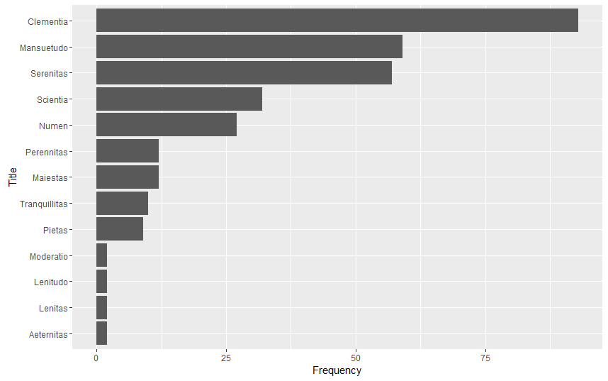
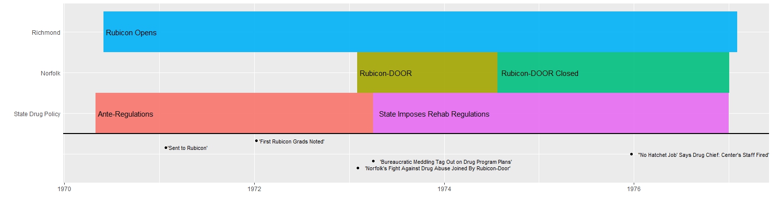
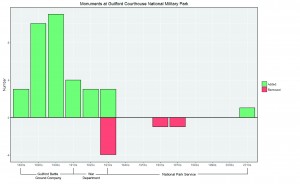
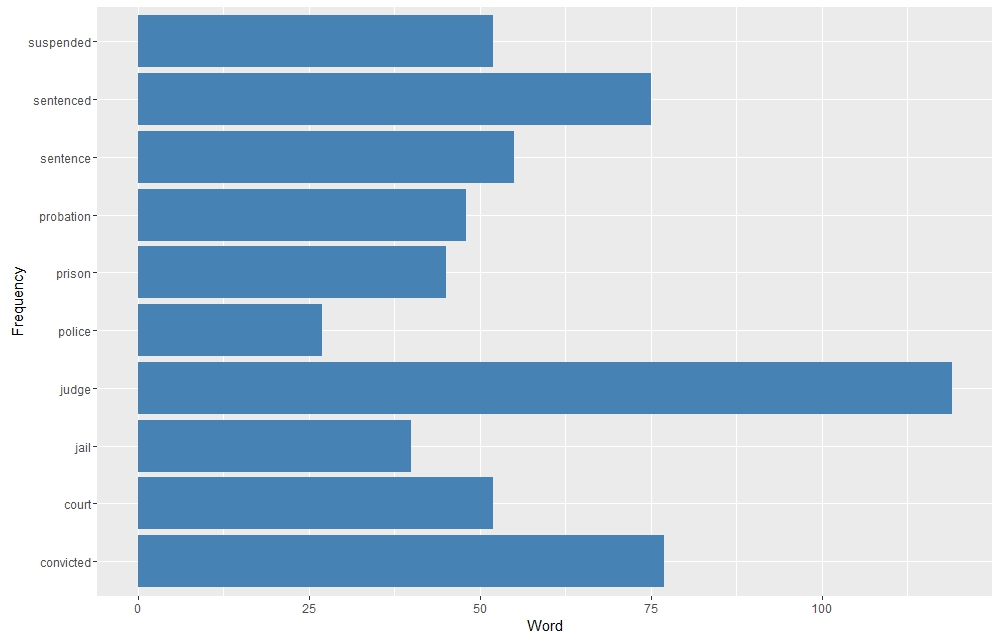
Using R I selected a few words that indicate Rubicon’s ties to the justice system. Over 66% of Rubicon’s clients were filtered through the justice system. As Indicated below words that exemplify this connection peaked in 1973, right when arrest numbers dropped across the state. Equally notable however is the sharp drop in 1974, which coincided with an increase in arrest numbers from 1973 to 1974. Rubicon either reached capacity or state drug control directives changed. As can be seen words like “probation” were not used continually over time and “convicted” and “sentence” drop out of favor too. This is probably due to a lack of space available at Rubicon after 1973.

rubline
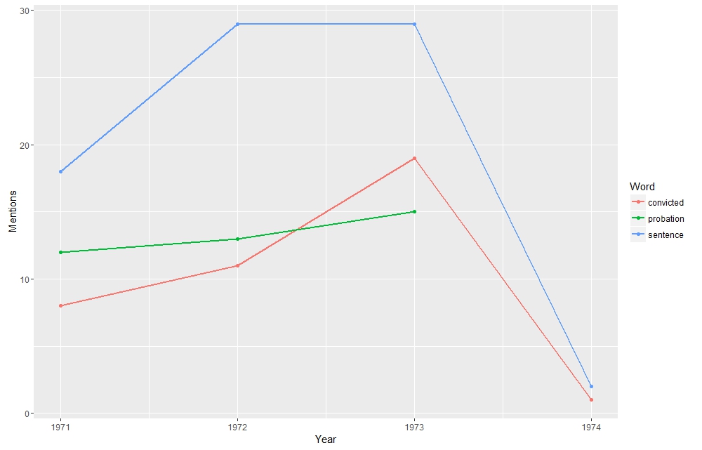
Sentiment Analysis of articles about Rubicon in three Virginia newspapers
sent-plot
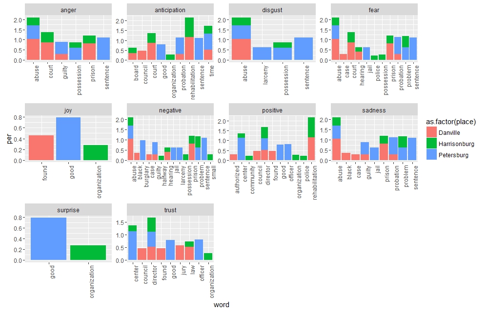
Word cluster of mentions of “police” within the Rubicon corpus. The city of Petersburg is heavily represented.

rubiconpoliceclus

Imperial Titles in Late Roman Documents

Sorry for the delay on my blog post! I’ve finally managed to figure out the coding to search for all inflections of the various nostra/mea epithets in Latin documents. I was having trouble using .*? to account for varying numbers of characters between nostra/mea and its accompanying noun (e.g. nostra clementia), as R was, despite the “?”, still being far too greedy. str_locate_all showed that it was pairing nostra‘s and titles that were thousands of characters apart!

My solution has been to ask R to search for combinations of nostra/mea and the accompanying noun with anywhere from 0 to 80 characters inbetween. Furthermore, I’ve simplified my code by only searching for the parts of these words that don’t inflect. So, for example, I wrote:

str_extract_all(string = CTh.df$text, pattern = “nostra.{0,80}clementia.{0,80}|clementia.{0,80}nostra.{0,80}|mea.{0,80}clementia.{0,80}|clementia.{0,80}mea.{0,80}”) #CLEMENTIA

This accounts for all inflections; it turns up nostra/mea clementianostrae/meae clementiae, and nostram/meam clementiam. I did this for all of the imperial epithets that I have identified within the Theodosian Code. I then used those results to locate and read each instance in the Latin text, both so as to confirm their use as imperial epithets within their respective contexts, and so as to record their exact location within the Code. It’s been time consuming, but very rewarding. I now have complete and accurate results for their frequency within the Code:

rplot

Now that I have an effective formula down, I will run through the rest of my documents this week: the main ones are the Code of Justinian, Symmachus’ Relationes to the emperors, and a series of Latin Panegyrics. I hope to have a few of these done before class on Thursday; I’ll update this post with those results.

My code

#THEODOSIAN CODE

CTh.scan <- scan(“~/Education/Emory/Coursework/Digital Humanities Methods/Project/Theodosian Code Raw Text.txt”,
what=”character”, sep=”\n”)
CTh.df <- data.frame(CTh.scan, stringsAsFactors=FALSE)
CTh.df <- str_replace_all(string = CTh.df$CTh.scan, pattern = “[:punct:]”, replacement = “”)
CTh.df <- data.frame(CTh.df, stringsAsFactors = FALSE)
CTh.lines <- tolower(CTh.df[,1])
book.headings <- grep(“book”, CTh.lines)
start.lines <- book.headings + 1
end.lines <- book.headings[2:length(book.headings)] – 1
end.lines <- c(end.lines, length(CTh.lines))
CTh.df <- data.frame(“start” = start.lines, “end”=end.lines, “text”=NA)
i <- 1
for (i in 1:length(CTh.df$end))
{CTh.df$text[i] <- paste(CTh.lines[CTh.df$start[i]:CTh.df$end[i]], collapse = ” “)}

CTh.df$Book <- seq.int(nrow(CTh.df))

#String Extracts of Imperial Titles

str_extract_all(string = CTh.df$text, pattern = “nostra.{0,80}aeternita.{0,80}|aeternita.{0,80}nostra.{0,80}|mea.{0,80}aeternita.{0,80}|aeternita.{0,80}mea.{0,80}”) #AETERNITAS

str_extract_all(string = CTh.df$text, pattern = “nostra.{0,80}clementia.{0,80}|clementia.{0,80}nostra.{0,80}|mea.{0,80}clementia.{0,80}|clementia.{0,80}mea.{0,80}”) #CLEMENTIA

str_extract_all(string = CTh.df$text, pattern = “nostra.{0,80}lenita.{0,80}|lenita.{0,80}nostra.{0,80}|mea.{0,80}lenita.{0,80}|lenita.{0,80}mea.{0,80}”) #LENITAS

str_extract_all(string = CTh.df$text, pattern = “nostra.{0,80}lenitud.{0,80}|lenitud.{0,80}nostra.{0,80}|mea.{0,80}lenitud.{0,80}|lenitud.{0,80}mea.{0,80}”) #LENITUDO

str_extract_all(string = CTh.df$text, pattern = “nostra.{0,80}maiesta.{0,80}|maiesta.{0,80}nostra.{0,80}|mea.{0,80}maiesta.{0,80}|maiesta.{0,80}mea.{0,80}”) #MAIESTAS

str_extract_all(string = CTh.df$text, pattern = “nostra.{0,80}mansuetud.{0,80}|mansuetud.{0,80}nostra.{0,80}|mea.{0,80}mansuetud.{0,80}|mansuetud.{0,80}mea.{0,80}”) #MANSUETUDO

str_extract_all(string = CTh.df$text, pattern = “nostra.{0,80}moderatio.{0,80}|moderatio.{0,80}nostra.{0,80}|mea.{0,80}moderatio.{0,80}|moderatio.{0,80}mea.{0,80}”) #MODERATIO

str_extract_all(string = CTh.df$text, pattern = “nostrum.{0,80}numen.{0,80}|numen.{0,80}nostrum.{0,80}|nostr.{0,80}numin.{0,80}|numin.{0,80}nostr.{0,80}|meum.{0,80}numen.{0,80}|numen.{0,80}meum.{0,80}|me.{0,80}numin.{0,80}|numin.{0,80}me.{0,80}”) #NUMEN

str_extract_all(string = CTh.df$text, pattern = “nostra.{0,80}perennita.{0,80}|perennita.{0,80}nostra.{0,80}|mea.{0,80}perennita.{0,80}|perennita.{0,80}mea.{0,80}”) #PERENNITAS

str_extract_all(string = CTh.df$text, pattern = “nostra.{0,80}pieta.{0,80}|pieta.{0,80}nostra.{0,80}|mea.{0,80}pieta.{0,80}|pieta.{0,80}mea.{0,80}”) #PIETAS

str_extract_all(string = CTh.df$text, pattern = “nostra.{0,80}scientia.{0,80}|scientia.{0,80}nostra.{0,80}|mea.{0,80}scientia.{0,80}|scientia.{0,80}mea.{0,80}”) #SCIENTIA

str_extract_all(string = CTh.df$text, pattern = “nostra.{0,80}serenita.{0,80}|serenita.{0,80}nostra.{0,80}|mea.{0,80}serenita.{0,80}|serenita.{0,80}mea.{0,80}”) #SERENITAS

str_extract_all(string = CTh.df$text, pattern = “nostra.{0,80}tranquillita.{0,80}|tranquillita.{0,80}nostra.{0,80}|mea.{0,80}tranquillita.{0,80}|tranquillita.{0,80}mea.{0,80}”) #TRANQUILLITAS

#Imperial Title Sums

aeternitas <- 2
clementia <- 93
lenitas <- 2
lenitudo <- 2
maiestas <- 12
mansuetudo <- 59
moderatio <- 2
numen <- 27
perennitas <- 12
pietas <- 9
scientia <- 32
serenitas <- 57
tranquillitas <- 10

#Imperial Title Sum Graph

Frequency <- c(clementia, mansuetudo, serenitas, scientia, numen, maiestas, tranquillitas, pietas, aeternitas, lenitas, lenitudo, moderatio)
Title <- c(“Clementia”, “Mansuetudo”, “Serenitas”, “Scientia”, “Numen”, “Maiestas”, “Tranquillitas”, “Pietas”, “Aeternitas”, “Lenitas”, “Lenitudo”, “Moderatio”)
sum.df <- cbind.data.frame(Title, Frequency)
sum.df$Title <- factor(sum.df$Title, levels = sum.df$Title[order(sum.df$Frequency)]) #Reorders dataframe based on Frequency

ggplot(data=sum.df, aes(x=Title, Frequency), y=Frequency) + geom_bar(stat = “identity”) + coord_flip() #Word Total Graph

Index of Imperial Epithets in the Theodosian Code

Nostra Aeternitas

10.22.3

Mea Aeternitas

12.1.160

Nostra Clementia

1.1.5
1.7.4
1.14.1
2.6.1
2.8.20
2.23.1
5.1.2
5.2.1
5.15.21
5.16.31
6.2.26
6.4.18
6.4.33
6.23.4
6.30.4
6.35.14
7.1.16
7.1.17
7.4.21
7.4.25
7.6.5
7.13.13
7.21.4
8.5.1
8.5.5
8.5.30
8.5.44
8.5.50
8.5.54
8.5.56
8.5.57
8.10.3
9.16.12
9.17.2
9.21.6
9.34.7
9.40.16
9.40.16
9.41.1
9.45.4
10.1.16
10.10.26
10.10.32
10.10.34
10.14.1
10.15.2
11.7.15
11.16.7
11.16.8
11.20.4
11.28.3
11.28.14
11.30.13
11.30.54
11.30.57
11.30.61
11.36.24
12.1.14
12.1.14
12.1.15
12.1.146
12.1.169
12.1.184
12.6.30
12.10.1
12.12.4
12.12.14
13.1.20
13.3.17
14.10.3
14.15.5
14.17.5
14.17.14
15.1.44
15.1.49
15.3.4
15.6.1
16.1.2
16.2.42
16.3.2
16.5.46
16.5.49
16.5.54
16.5.54
16.5.60
16.5.63
16.8.17
16.11.2

Mea Clementia

1.8.2
1.8.3
6.26.17
7.16.2
11.20.5

Nostra Lenitas

1.22.2
10.8.3

Nostra Lenitudo

8.12.6
15.1.5

Nostra Maiestas

6.21.1
6.27.17
6.27.17
8.4.26
8.5.39
11.29.1
11.30.66
11.30.68
13.3.18
14.3.18
15.1.47
16.10.20

Nostra Mansuetudo

1.2.8
1.5.9
1.10.1
1.15.8
1.28.1
3.9.1
4.14.1
6.2.19
6.22.8
6.23.4
6.30.18
6.30.20
7.13.9
8.5.12
8.5.22
8.5.54
8.5.58
8.8.2
8.10.2
9.16.10
9.30.2
10.7.2
10.7.2
10.9.2
10.9.3
10.10.20
10.16.2
11.7.21
11.12.4
11.16.11
11.16.14
11.28.3
11.28.5
11.30.32
11.30.41
11.30.41
12.6.5
12.6.12
12.6.28
12.12.5
12.12.10
12.12.10
12.19.3
13.3.4
13.5.38
13.6.5
14.1.2
14.4.3
14.9.1
15.3.1
15.5.5
15.7.4
15.7.6
15.7.9
16.2.12
16.5.7
16.5.38
16.10.2

Mea Mansuetudo

12.1.121

Nostra Moderatio

6.30.24
8.18.3

Nostrum Numen

1.2.12
1.9.2
2.23.1
2.33.4
5.12.3
5.12.3
6.4.29
6.4.32
6.5.2
6.14.3
6.23.3
6.30.15
7.7.4
7.8.3
8.1.13
8.5.40
8.5.62
9.40.11
11.21.3
11.28.15
11.30.49
12.12.7
15.4.1
15.5.5
16.4.4
16.8.13

Meum Numen

11.1.33

Nostra Perennitas

1.1.5
2.4.4
4.4.5
5.15.18
7.7.4
9.19.3
9.38.8
10.20.10
12.12.9
13.5.12
15.1.31

Mea Perennitas

6.30.21

Nostra Pietas

5.12.3
6.10.1
10.26.1
11.1.34
11.1.36
13.1.21
14.26.2
15.1.37

Mea Pietas

14.16.2

Nostra Serenitas

1.1.2
1.12.5
1.22.2
2.16.2
4.4.3
5.13.2
5.16.31
6.8.1
6.22.3
6.23.1
6.26.13
6.27.8
6.29.3
6.30.17
7.1.17
7.8.10
8.5.14
8.5.22
8.5.32
8.5.45
8.5.48
8.5.56
8.7.16
9.19.3
9.38.6
9.38.9
9.40.7
9.40.20
9.42.14
9.42.19
9.42.20
10.10.11
11.2.5
11.16.20
11.28.4
11.30.47
11.30.56
11.30.64
11.31.9
11.31.9
12.13.6
13.10.8
14.2.1
14.4.8
15.1.11
15.1.26
15.1.42
15.1.51
15.5.5
15.7.6
15.7.6
16.2.37
16.5.12
16.5.14
16.8.22
16.11.3

Mea Serenitas
11.20.5

Nostra Scientia

1.1.5
1.5.1
1.15.2
1.16.6
1.29.1
2.18.1
6.4.21
7.1.12
8.5.25
9.1.1
9.1.13
9.4.1
9.21.1
9.34.3
10.8.3
11.7.16
11.16.8
11.16.8
11.29.2
11.30.1
11.30.1
11.30.9
11.30.18
11.30.18
11.37.1
12.1.1
12.12.3
15.1.2
15.1.2
15.1.30
16.10.1
16.10.15

Nostra Tranquillitas

1.2.10
1.6.4
5.15.18
6.4.31
6.12.1
8.7.16
11.30.31
16.1.4
16.2.15
16.4.1


Historiographical Research on Natsume Soseki and Dazai Osamu

Plan for Final Research Project

For the final research, I am going to analyze the works of the early 20th century Japanese writers. I want to choose two to three authors from Natsume Soseki, Dazai Osamu, Tanizaki Junichiro and Akutagawa Ryunosuke, so the project will not be too overwhelming. Many of their work are available on Aozora Bunko, and I have read at least one of their work.

Historiographical Research

The Data for Research of JSTOR is not a perfect tool for historiographical research on Japanese literature. My search for the keyword “Nastume Soseki” gives back a two documents on Shakespeare in 2000 and 2001.

shakespeare
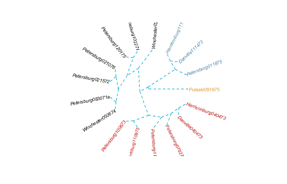
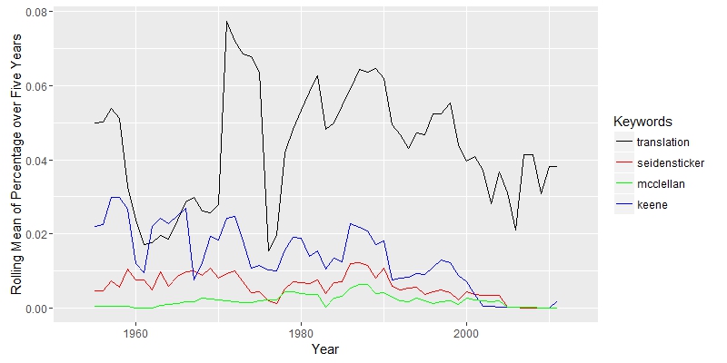
These outliers, however, are not going to seriously affect the study, since I am only interested in counting word frequency and I have a large data set. The code I used is from class. I wrote some new code for graphing and picking frequent word from the document.

The key term “Nastume Soseki” yields a result of 697 documents. For the vertical axis in all the following graphs, I used rolling mean of percentage of the word over five years, since it gives the most smooth graph.

Group 1: Translation

Since the majority of documents from JSTOR are in English, I expected many documents to discuss translation. The first group of keywords that I looked for is “translation” and names of three famous translators.natsume-soseki-translation
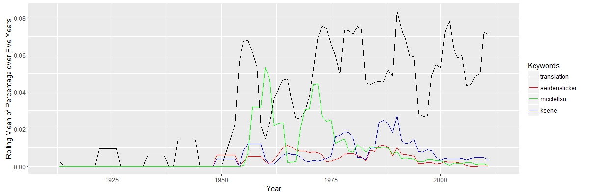
The graph shows that the study of Nastume Soseki’s work in translation rise around 1950. It makes sense, since most of his work was translated after World War II. There are only a few document before 1950 in the result. The key term “translation”, although with some fluctuation, is always important after 1950. Three other keywords “McClellan”, “Keene” and “Seidensticker”, translators’ names, appeared more from 1950 to 2000. The three authors were all born in 1920s, so their works concentrated in the late 20th century.

Group 2: Language

natsume-soseki-language
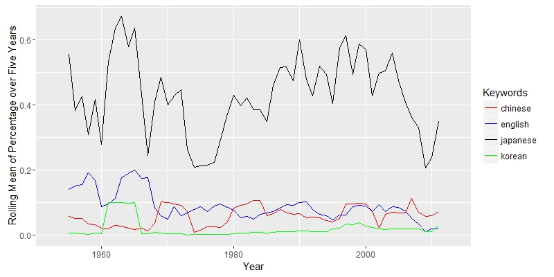
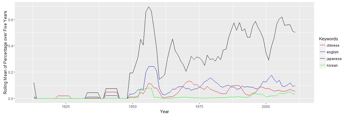
The keyword “Japanese” appeared dominant as expected. Because most of the documents are from Asian studies journals, “Chinese” and “Korean” appears frequently. The line of “English” is close to the line of “Chinese”. If most of works are about translation, the word “English” would appear more. Therefore, there maybe a large portion of the work that does not directly discuss translation; these documents are probably about general literature or cultural study.

GROUP 3: Theme
natsume-soseki-theme

The four key words in these graph are “death”, “love”, “moral” and “war”. “Love” and “war” are more prevalent. “War” also appears in works published during WWII, and have several peaks. I do not remember reading a lot about war in Natsume Soseki’s works, but scholars might what to find what is the connection between pre-war literature and WWII. I find “war” is similarly a dominant key term in the search for “Dazai Osamu” in DfR in JSTOR, although most of his work are not related to war.

Group 4: IMPLICATION AND CONNECTION

natsume-soseki-discipline
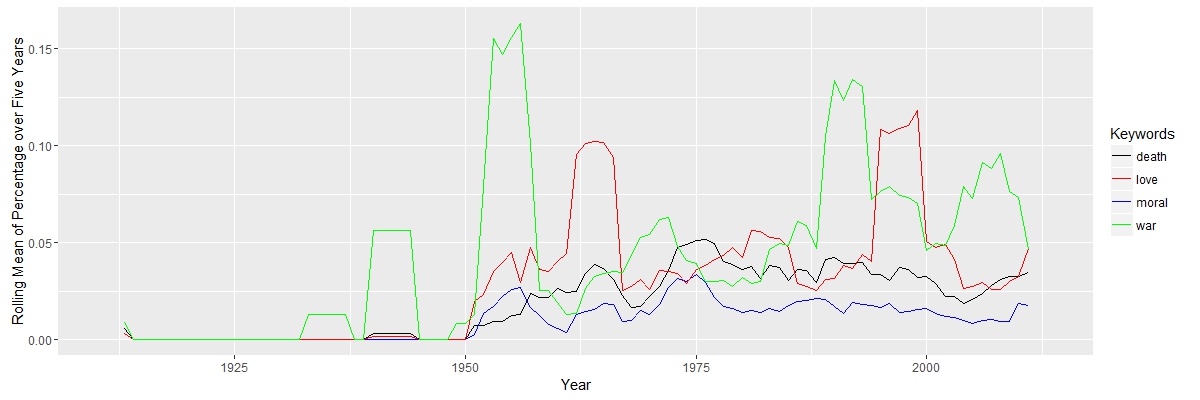
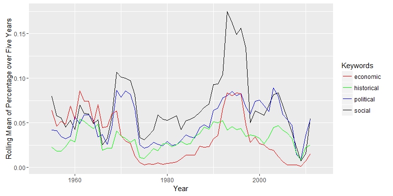
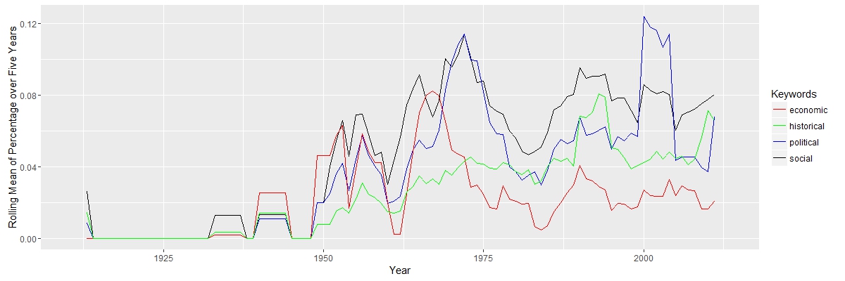
Here, I am interested in how scholars interpreted Natsume’s works and their political, social, economic and historical connections. “Political” and “social” are closely related, since they move together. “Economic” has a falling importance, while “historical” appeared to be more import along the timeline.

GROUP 5: AUTHORS

natsume-soseki-authors
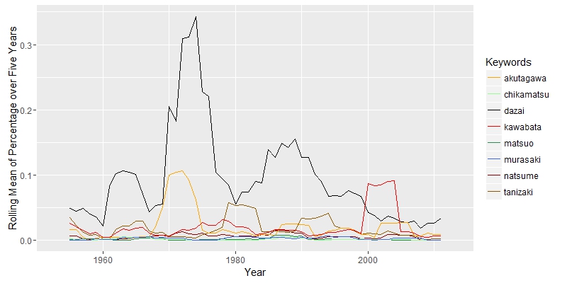
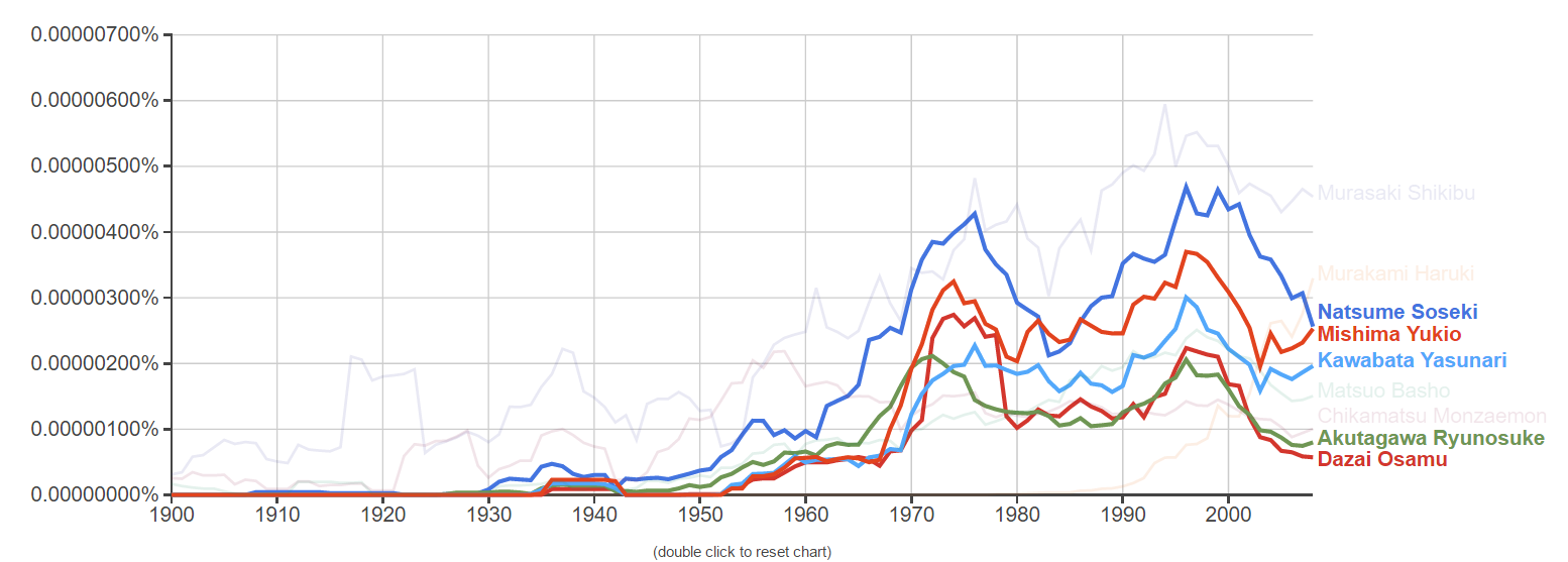
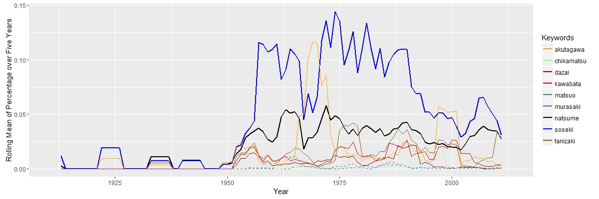
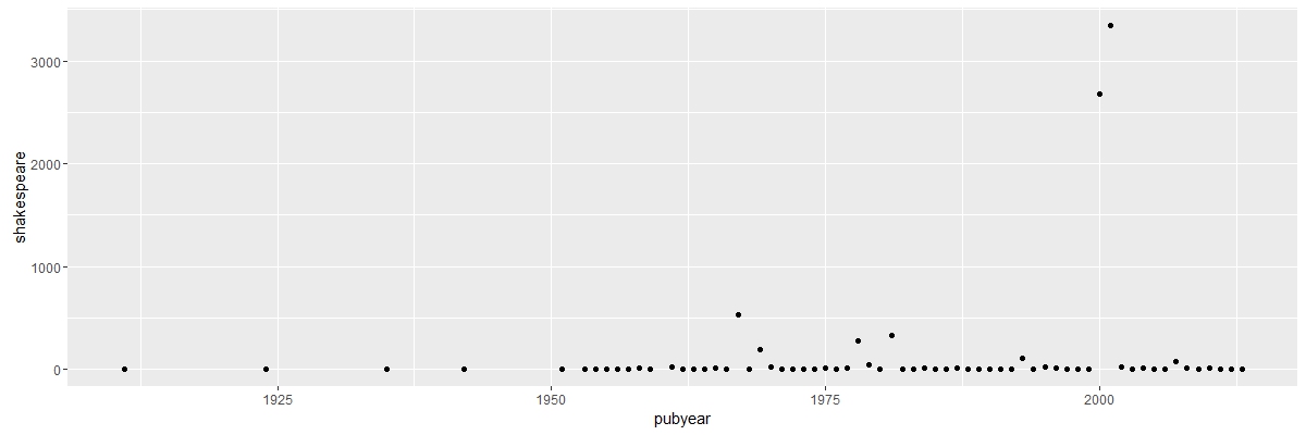
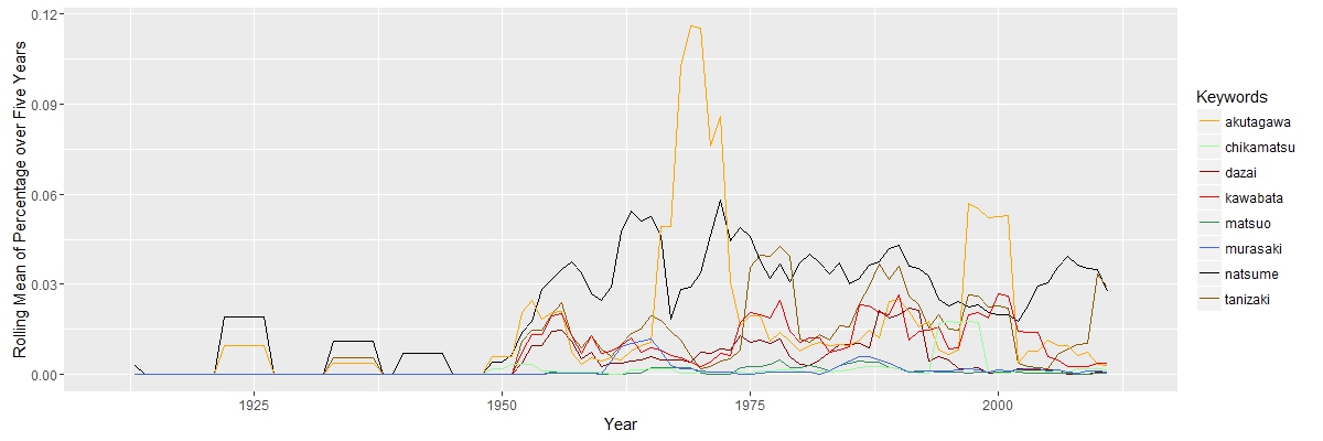
The search for “Natsume Soseki” in JSTOR does not return documents exclusively about Natsume Soseki. Some documents about other Japanese authors may also appear. The graph above shows that “natsume” was constantly above other authors, except years aroud 1965 and 2000, when “akutagawa” has two peaks. The truth is that “akutagawa” appears in total 109 times from 1968 to 1972 and 153 times in 2004. The data set is not perfect, but it will not cause serious bias.

The graph also shows the correlation between authors. Three of the authors, “murasaki”, “chikamatsu” and “matsuo”, are not from the 20th century. Their lines are in green and blue and do not raise much from 0. Modern authors, whose lines are in orange and red. The line for “tanizaki”, “dazai”and “kawabata” are close together.

Similar Graph for the Search of Dazai Osamu

dazai-osamu-translation

“Keene” is more important among the three translator. He translated Dazai’s “No Longer Human”.

dazai-osamu-languagedazai-osamu-theme

“War” is also a dominant theme, but the peaks around 1960 and 2000 are somewhat different in time from the previous graph from Nastume Soseki.

dazai-osamu-displinedazai-osamu-author

This graph looks better, since “dazai” is more dominant.

Google Ngram

Google Ngram is easy to use and its results are interesting.

ngram1

All five are the 20th century Japanese writers. From this graph, we can see the frequency increased from 1950, and have two peaks at 1970s and 1990s. This partially match the graph of Dazai, but is different from the graph of Natsume from JSTOR.

ngram2

Three ancient writers, Murasaki (11th c.), Matsuo(17th c.) and Chikamatsu(17th c.) do not follow the pattern of 20th century writers.

ngram3

Contemporary writers, Murakami (1949 – ) do not follow the pattern as well.

Part of the code for PLOtting

I have difficulty changing the order of the legends, but everthing else works fine.

keepers <- c("japanese","english","chinese","korean")
Tokugawa.full.smaller <- Tokugawa.full.perc.df[,keepers]
Tokugawa.full.smaller[is.na(Tokugawa.full.smaller)] <- 0
Tokugawa.smaller.roll.5 <- data.frame(rollmean(Tokugawa.full.smaller, k=5, fill = list(NA, NULL, NA)))
Tokugawa.smaller.roll.5$pubyear <- Tokugawa.full.perc.df$pubyear
mathching <- c("japanese" = "black","english" = "blue","chinese" = "red","korean" = "green")
ggplot(Tokugawa.smaller.roll.5, aes(x=pubyear)) + 
 geom_line(aes(y = japanese, color = "japanese")) +
 geom_line(aes(y = english, color = "english"))+
 geom_line(aes(y = chinese, color = "chinese")) +
 geom_line(aes(y = korean, color = "korean")) +
 scale_colour_manual(name="Keywords",values = mathching)+
 xlab("Year") + ylab("Rolling Mean of Percentage over Five Years")