Author: Zixuan Li

A Short Introduction of Natsume Soseki

Natsume Soseki, born in 1867, the year before the Meiji Restoration, was a Japanese author whose works characterized the perplexity of Japanese during the era of rapid westernization. He loved Chinese literature, but studying English was a fashion at his time. Therefore, he became a scholar in English literature. The Japanese government sent him to study in England from 1901 to 1903, but this became his most unpleasant years. Soseki became mad in London, and started to question the idea of modernity. He was aware of the superficiality of Japanese westernization and aimless imitation of the west. In his works, he mainly focused on the pain and solitude that modernity brought to Japanese. Between 1905 and 1916, he wrote fifteen novels, including one unfinished. In 1907, Soseki rejected his professorship and started to work for Asahi newspaper, where most of his works were published. In 1916, he died of stomach ulcer.

Update on Historiographical Research

This is an update on last post. Natsume Soseki is commonly referred by his given name (or rather pen name), Soseki, so searching for “Soseki” in DfR of JSTOR collections is more accurate.

Text Mining of Soseki’s Novels

The central question that I am asking is what issues on modernity and tradition did Soseki write about and was Soseki more inclined to the traditional side or modern side.

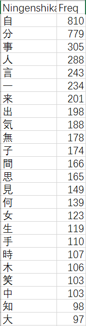
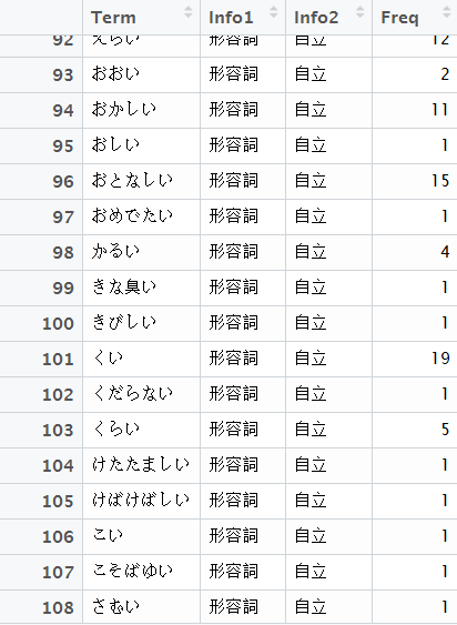
The Japanese tokenizer MeCab with IPA dictionary takes in a txt file and produces a dataframe like the following graph. Term column is the word. Info1 is part of speech. Info2 is more information on part of speech.

I processed the txt files with the same code I did a month ago, taking out pronunciation guide and style annotations. Then, I used dataframes generated by MeCab to calculate the term frequency in percentage and tf-idf. For all the graphs, the novels names on the axes are in chronological order

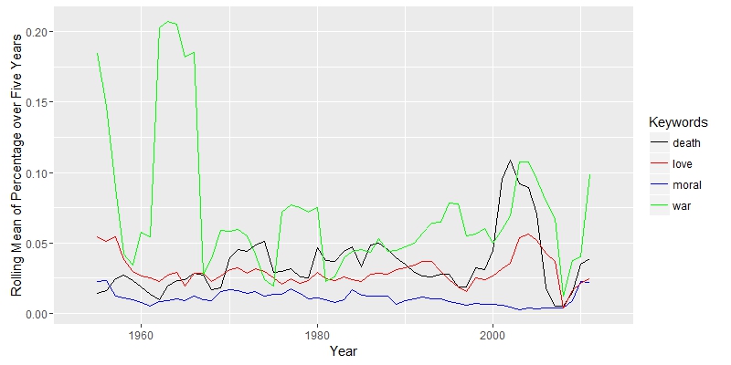
First, I focused on term frequency of some keywords. In last post I mentioned that English scholars were interested in discussion wars in studies of Japanese literature. This interests are not unjustified, since most of Soseki’s works mentioned words related to military and war. Meiji Japan was also a time of military victories, like Sino-Japanese War (1894-95) and Russo-Japanese War (1904-05). These were directly related to the westernization of Japan.

Nevertheless, the word related to war was not that common compared to words related to love or death. In some of the works, Soseki showed his idea on love and solitude in modern world and how marriage in the new era should be different from old time. Maybe scholars should pay more attention to these issues.

For the other question, how did Soseki place himself in modernity and tradition. Although some famous critic, like Eto Jun thinks that Soseki stands on the side of tradition, especially in his last several works, more scholars argue that Soseki stands on side of modernity. Soseki was aware of the pain brought by westernization to Japanese, but he did not deny it. In some of his essays, he justified Japanese colonization of Manchuria and Korea by commenting that this was an inevitable result of a modernizing Japan.

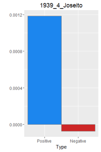
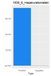
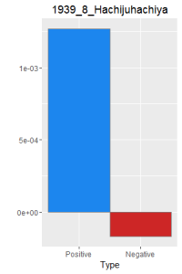
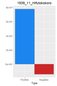
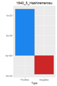
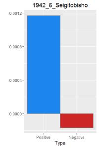
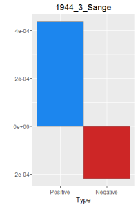
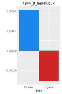
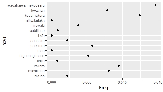
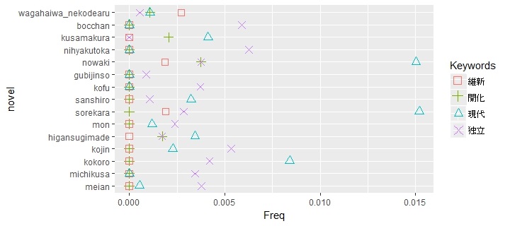
The following figure presents frequency of four words, restoration (維新), enlightenment (開化), modernity (現代) and independent (独立), directly related to modernity and Meiji Restoration, in his novels. All of the novels used at least one of the four words.
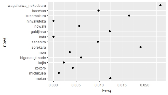
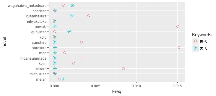
The following graph is a comparison between the frequencies the word modernity (現代) and antiquity (古代).Soseki used a lot more modernity than antiquity.  I wanted to find the frequency of tradition (伝統) or national learning (国学), but it turned out that Soseki never used these words.

It might be the case that words like tradition or national learning emphasize superiority of Japanese culture, so Soseki avoided using them. His was disgusted by shallow nationalist movement of his classmates when he was young. By contrast the word Chinese study appeared several time in his novels.

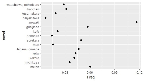
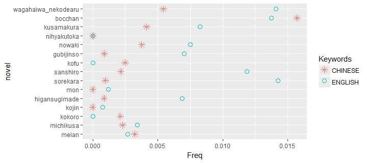
Another way of looking at the question is to search for the words related to Chinese and English. For Soseki, Chinese is the more traditional culture and English is more modern, while the westernizing Japan is somewhere between modernity and tradition. Related words to Chinese include Qing Empire (清国), Japan-Qing (日清), China (中国), Chinese book (漢籍), Chinese land (漢土) and Chinese poetry (漢詩); related words to English include the UK (イギリス or 英国), English (英語 or 英文), Anglo-Japanese (英和) and English translation (英訳)

This graph is not as extreme as last one. Although words related to English is still more important, words related to Chinese appear a lot.

Tf-idf

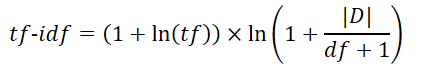
The above equation is what I used for tf-idf. Both term frequency and document frequency are normalized.

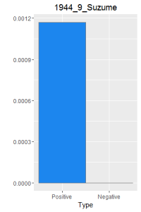
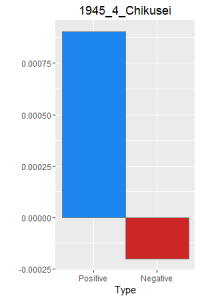
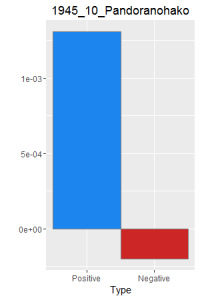
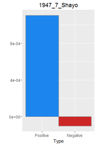
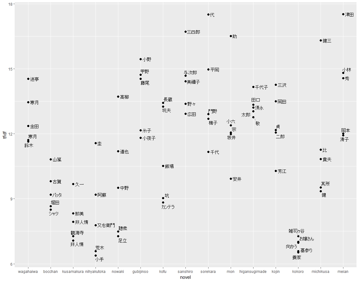
Some of the novels are more interesting than other. Kokoro (The Hearts) is one of Soseki’s most beloved novel. The following graph is the top 5 words by tf-idf for each novel. Kokoro has the lowest tf-idf index, because it does not use many uncommon word. In other novels, characters has names, so the names have high tf-idf index. However, Soseki is reluctant to give characters names in Kokoro, so the most distinctive word is Zoshigaya (雑司ヶ谷), which is a place name in Tokyo.

Edwin McClellan, who introduced Soseki to western audience and translated two of Soseki’s novels, comments that Soseki wrote Kokoro as an “allegory of sorts”. Isolation and pain of Sensei, the protagonist in Volumn 3 of Kokoro, could be troubles to any Meiji intellectuals. The work is not only stylistically simple as noted by McClellan, but also lexically simple as shown in following graphs.

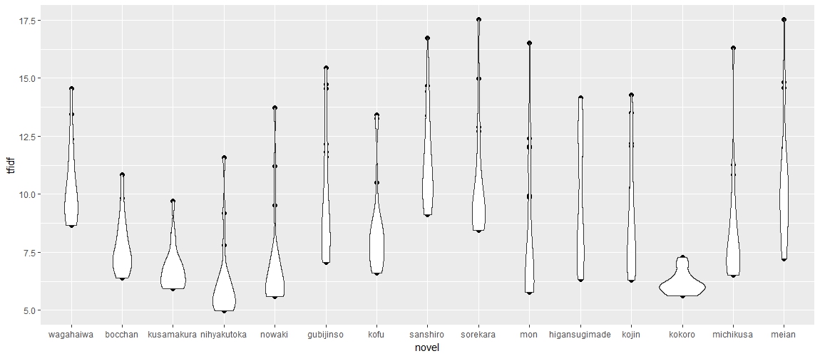
A violin graph of top 20 words by tf-idf also shows that Kokoro tends to use common word.

Code

### Text Processing code is in the post about Dazai Osamu

### Make frequency tables with RMeCab

Sys.setlocale(“LC_ALL”, “Japanese”) ### Windows users may want to use this to avoid encoding problems

library(RMeCab) ### Japanese Tokenizer

na.zzz <- RMeCabFreq(“D:/Google Drive/JPN_LIT/Natsume/zzz.txt”)
na.zzz.reduced <- na.zzz[which(na.zzz$Info1 != “記号”),] ###Take out punctuations

files.cle.dir<- list.files(“D:/Google Drive/JPN_LIT/Natsume/cleaned”)

for (n.i in 1:length(files.cle.dir)){
assign(paste0(“n.”, files.cle.dir[n.i]), RMeCabFreq(paste0(“D:/Google Drive/JPN_LIT/Natsume/cleaned/”,files.cle.dir[n.i]))[which(RMeCabFreq(paste0(“D:/Google Drive/JPN_LIT/Natsume/cleaned/”,files.cle.dir[n.i]))$Info1 != “記号”),])
}

###A sample code of combining frequency table of a novel to the frequency table of the corpus of fifteen novels.

z <- 1
y <- 1
while (z <= length(na.zzz.reduced$Term)){
if(n.bocchan.txt$Term[y] == na.zzz.reduced$Term[z] & n.bocchan.txt$Info1[y] == na.zzz.reduced$Info1[z] & n.bocchan.txt$Info2[y] == na.zzz.reduced$Info2[z]){
na.zzz.reduced$bocchan[z] <- n.bocchan.txt$Freq[y]
y <- y + 1
}
z <- z + 1
}

### na.zzz.reduced is the final frequency dataframe with every novel

### Tf-idf

n.TMD <- na.zzz.reduced[,4:19]
n.TMD$Dfreq <- apply(n.TMD, 1, function(x) length(which(x != 0)))
n.TMD$Dfnorm <- log(15/n.TMD$Dfreq +1)

n.TFIDF.df <- data.frame(t(apply(n.TMD[,2:16], 1, function(x) log(x)+1)))
n.TFIDF.df <- n.TFIDF.df*n.TMD$Dfnorm
n.TFIDF.df[n.TFIDF.df == -Inf] <- 0

Final.TFIDF.df <- cbind(na.zzz.reduced[,1:3],n.TFIDF.df)

##### Make another table of Final percentage

n.PERC.df<- data.frame(apply(n.TMD[,1:16], 2,function(x) x/sum(x)*100))
Final.PERC.df <- cbind(na.zzz.reduced[,1:3],n.PERC.df)

 

###Make a dataframe of top 20 and top 5 tfidf for each novel and change the name of wagahaiwa_nekodearu since it is too long
all.TFIDF20 <- data.frame(Term = NA,tfidf = NA, novel = NA)
for (col.i in 4:18){
all.TFIDF20 <- rbindlist(list(all.TFIDF20, cbind(Final.TFIDF.df[order(-Final.TFIDF.df[,col.i]),][1:20,][,c(1,col.i)],colnames(Final.TFIDF.df)[col.i])))
}
all.TFIDF20 <- all.TFIDF20[-1,]
all.TFIDF20$novel <- as.character(all.TFIDF20$novel)
all.TFIDF20[all.TFIDF20 == “wagahaiwa_nekodearu”] <- “wagahaiwa”

### Top5 tf-idf

all.TFIDF5 <- data.frame(Term = NA,tfidf = NA, novel = NA)
for (col.i in 4:18){
all.TFIDF5 <- rbindlist(list(all.TFIDF5, cbind(Final.TFIDF.df[order(-Final.TFIDF.df[,col.i]),][1:5,][,c(1,col.i)],as.character(colnames(Final.TFIDF.df)[col.i]))))
}
all.TFIDF5 <- all.TFIDF5[-1,]
all.TFIDF5$novel <- as.character(all.TFIDF5$novel)

### Violin Graph

ggplot(all.TFIDF20, aes(x = novel, y = tfidf))+
geom_point(size = 2) +
scale_x_discrete(limits=c(“wagahaiwa”,”bocchan”,”kusamakura”,”nihyakutoka”,”nowaki”,”gubijinso”,”kofu”,”sanshiro”,”sorekara”,”mon”,”higansugimade”,”kojin”,”kokoro”,”michikusa”,”meian”)) +
geom_violin()

### Top 5 tf-idf with term shown

library(ggrepel) ### An extension to ggplot2 to avoid overlap of terms in graph

ggplot(all.TFIDF5, aes(x = novel, y = tfidf))+
geom_point(size = 2) +
scale_x_discrete(limits=c(“wagahaiwa”,”bocchan”,”kusamakura”,”nihyakutoka”,”nowaki”,”gubijinso”,”kofu”,”sanshiro”,”sorekara”,”mon”,”higansugimade”,”kojin”,”kokoro”,”michikusa”,”meian”)) +
geom_text_repel(aes(label=Term), size =4, segment.color = ‘grey60’,nudge_x =0.05)

### A sample graph of how I made the table for words related to Chinese and English. All other frequency graphs are similar (I admit that I used Mspaint to change some of the legend, because it is more convenient)
chn.all.PERC.df <- Final.PERC.df[which(Final.PERC.df$Term == “清国” |
Final.PERC.df$Term == “中国”|
Final.PERC.df$Term == “漢学”|
Final.PERC.df$Term ==”漢語”|
Final.PERC.df$Term ==”漢詩”|
Final.PERC.df$Term ==”漢籍”|
Final.PERC.df$Term ==”漢土”|
Final.PERC.df$Term ==”漢”|
Final.PERC.df$Term ==”漢人”),] ### I choose the terms based on search for three words, “清”, “漢” and “中国”.

eng.all.PERC.df <- Final.PERC.df[which(Final.PERC.df$Term == “イギリス” |
Final.PERC.df$Term == “英国”|
Final.PERC.df$Term == “英訳”|
Final.PERC.df$Term ==”英語”|
Final.PERC.df$Term ==”英文”|
Final.PERC.df$Term ==”英和”),]### The choice of vocabularies is similarly determined by the research intention
chn.eng.df <- data.frame(apply(chn.all.PERC.df[,5:19], 2, function(x) sum(x)))
chn.eng.df <- cbind(chn.eng.df, data.frame(apply(eng.all.PERC.df[,5:19], 2, function(x) sum(x))))

colnames(chn.eng.df) <- c(“CHINESE”, “ENGLISH”)

chn.eng.df$novel <- row.names(chn.eng.df)

ggplot(chn.eng.df, aes(x = novel))+
geom_point(aes(y=CHINESE, color = “CHINESE”), shape = 8, size =3) +
geom_point(aes(y=ENGLISH, color = “ENGLISH”), shape = 1, size =3) +
scale_x_discrete(limits=rev(c(“wagahaiwa_nekodearu”,”bocchan”,”kusamakura”,”nihyakutoka”,”nowaki”,”gubijinso”,”kofu”,”sanshiro”,”sorekara”,”mon”,”higansugimade”,”kojin”,”kokoro”,”michikusa”,”meian”))) +
labs(color=”Keywords”)+
ylab(“Freq”) +
coord_flip()

Plan for Final Research Project

For the final research, I am going to analyze the works of the early 20th century Japanese writers. I want to choose two to three authors from Natsume Soseki, Dazai Osamu, Tanizaki Junichiro and Akutagawa Ryunosuke, so the project will not be too overwhelming. Many of their work are available on Aozora Bunko, and I have read at least one of their work.

Historiographical Research

The Data for Research of JSTOR is not a perfect tool for historiographical research on Japanese literature. My search for the keyword “Nastume Soseki” gives back a two documents on Shakespeare in 2000 and 2001.

These outliers, however, are not going to seriously affect the study, since I am only interested in counting word frequency and I have a large data set. The code I used is from class. I wrote some new code for graphing and picking frequent word from the document.

The key term “Nastume Soseki” yields a result of 697 documents. For the vertical axis in all the following graphs, I used rolling mean of percentage of the word over five years, since it gives the most smooth graph.

Group 1: Translation

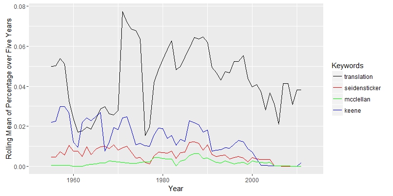
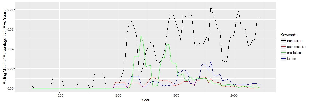
Since the majority of documents from JSTOR are in English, I expected many documents to discuss translation. The first group of keywords that I looked for is “translation” and names of three famous translators.The graph shows that the study of Nastume Soseki’s work in translation rise around 1950. It makes sense, since most of his work was translated after World War II. There are only a few document before 1950 in the result. The key term “translation”, although with some fluctuation, is always important after 1950. Three other keywords “McClellan”, “Keene” and “Seidensticker”, translators’ names, appeared more from 1950 to 2000. The three authors were all born in 1920s, so their works concentrated in the late 20th century.

Group 2: Language

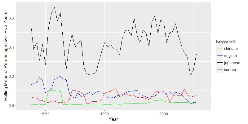
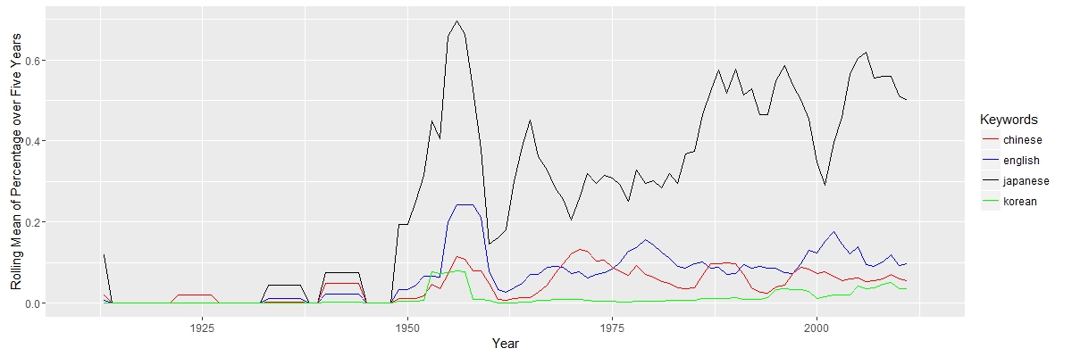
The keyword “Japanese” appeared dominant as expected. Because most of the documents are from Asian studies journals, “Chinese” and “Korean” appears frequently. The line of “English” is close to the line of “Chinese”. If most of works are about translation, the word “English” would appear more. Therefore, there maybe a large portion of the work that does not directly discuss translation; these documents are probably about general literature or cultural study.

GROUP 3: Theme

The four key words in these graph are “death”, “love”, “moral” and “war”. “Love” and “war” are more prevalent. “War” also appears in works published during WWII, and have several peaks. I do not remember reading a lot about war in Natsume Soseki’s works, but scholars might what to find what is the connection between pre-war literature and WWII. I find “war” is similarly a dominant key term in the search for “Dazai Osamu” in DfR in JSTOR, although most of his work are not related to war.

Group 4: IMPLICATION AND CONNECTION

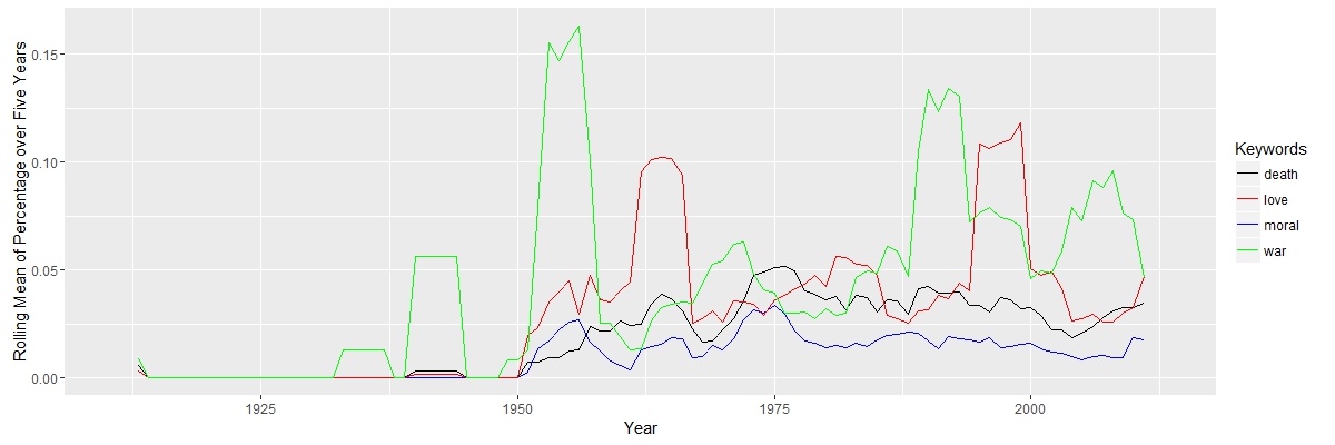
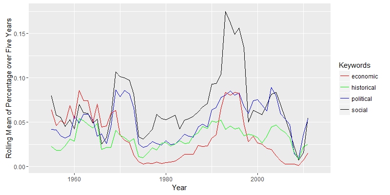
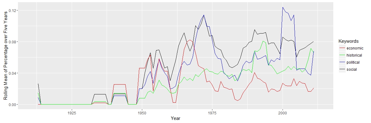
Here, I am interested in how scholars interpreted Natsume’s works and their political, social, economic and historical connections. “Political” and “social” are closely related, since they move together. “Economic” has a falling importance, while “historical” appeared to be more import along the timeline.

GROUP 5: AUTHORS

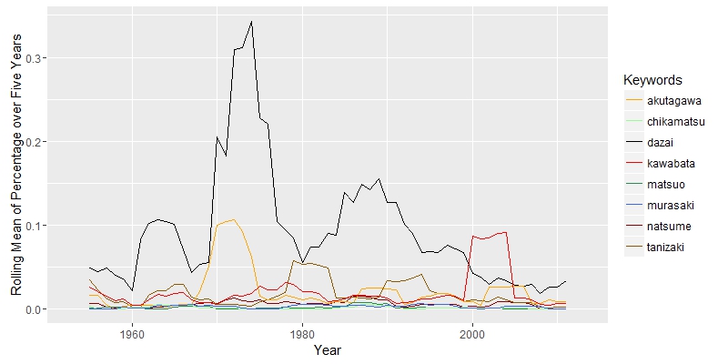
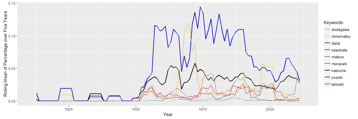
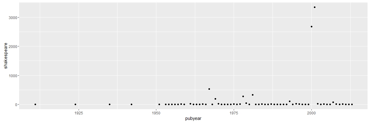
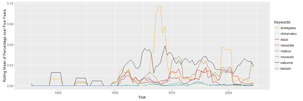
The search for “Natsume Soseki” in JSTOR does not return documents exclusively about Natsume Soseki. Some documents about other Japanese authors may also appear. The graph above shows that “natsume” was constantly above other authors, except years aroud 1965 and 2000, when “akutagawa” has two peaks. The truth is that “akutagawa” appears in total 109 times from 1968 to 1972 and 153 times in 2004. The data set is not perfect, but it will not cause serious bias.

The graph also shows the correlation between authors. Three of the authors, “murasaki”, “chikamatsu” and “matsuo”, are not from the 20th century. Their lines are in green and blue and do not raise much from 0. Modern authors, whose lines are in orange and red. The line for “tanizaki”, “dazai”and “kawabata” are close together.

Similar Graph for the Search of Dazai Osamu

“Keene” is more important among the three translator. He translated Dazai’s “No Longer Human”.

“War” is also a dominant theme, but the peaks around 1960 and 2000 are somewhat different in time from the previous graph from Nastume Soseki.

This graph looks better, since “dazai” is more dominant.

Google Ngram

Google Ngram is easy to use and its results are interesting.

All five are the 20th century Japanese writers. From this graph, we can see the frequency increased from 1950, and have two peaks at 1970s and 1990s. This partially match the graph of Dazai, but is different from the graph of Natsume from JSTOR.

Three ancient writers, Murasaki (11th c.), Matsuo(17th c.) and Chikamatsu(17th c.) do not follow the pattern of 20th century writers.

Contemporary writers, Murakami (1949 – ) do not follow the pattern as well.

Part of the code for PLOtting

I have difficulty changing the order of the legends, but everthing else works fine.

keepers <- c("japanese","english","chinese","korean")
Tokugawa.full.smaller <- Tokugawa.full.perc.df[,keepers]
Tokugawa.full.smaller[is.na(Tokugawa.full.smaller)] <- 0
Tokugawa.smaller.roll.5 <- data.frame(rollmean(Tokugawa.full.smaller, k=5, fill = list(NA, NULL, NA)))
Tokugawa.smaller.roll.5$pubyear <- Tokugawa.full.perc.df$pubyear
mathching <- c("japanese" = "black","english" = "blue","chinese" = "red","korean" = "green")
ggplot(Tokugawa.smaller.roll.5, aes(x=pubyear)) + 
 geom_line(aes(y = japanese, color = "japanese")) +
 geom_line(aes(y = english, color = "english"))+
 geom_line(aes(y = chinese, color = "chinese")) +
 geom_line(aes(y = korean, color = "korean")) +
 scale_colour_manual(name="Keywords",values = mathching)+
 xlab("Year") + ylab("Rolling Mean of Percentage over Five Years") 

 

Background

Dazai Osamu (太宰 治) is a 20th-century Japanese novelist. Many of his works centers around mental illness and darkness of human nature, emitting abject or even morbid emotions. His most famous work include Run, Melos! (走れメロス), The Setting Sun, (斜陽) and No Longer Human, (人間失格). He committed suicide in 1948.

The text comes from Aozora Bunko (青空文庫), which is the Japanese Project Gutenberg. I downloaded the txt form of the works, but it is not cleaned as the txt from Project Gutenberg. I have to take out the ruby (inside《》, 笑《わら》う), Japanese pronunciation notation , the notation of the editor (inside［］,［＃「ファン」に傍点］), and “｜” for separation in various conditions.

After cleaning these notation and white space, I first made a character frequency table of Ningen Shikkaku (No Longer Human). I admit I did this manually, chopping the text into single characters and kana, making the frequency table and deleting all kana. If there is a regex expression for kana in R, it will make this work easier.

Here is the first 25 most frequent character in Ningen Shikkaku

One thing I find intriguing thing about this table is that in such a morbid and hopeless novel like Ningen Shikkaku, Dazai Osamu used the character for laugh (笑) for 103 times, 22nd of all characters.  This lead me to look closely into the character and possible vocabularies and conjugations that it forms.

Challenge of Tokenization

The challenge is tokenization. There are many great tools available online, but it takes time to learn to use them, and I do not know if they will work with long text. Therefore, for this week’s text, I used simple code to divide characters and kana into groups of same length. This does not directly solve the problem of tokenization, but rather goes around it.

Here is an example of the code for creating groups of length 2:

g2 <- 2
Text.cleaned.split.group2 <- paste(Text.cleaned.split[1:2], collapse = "")
     for (g2 in 2:(length(Text.cleaned.split) - 1)){
     group2 <- paste(Text.cleaned.split[g2:(g2+1)], collapse = "")
     Text.cleaned.split.group2 <- c(Text.cleaned.split.group2,group2)
}

The code runs so slowly, taking more than 10 seconds for a novel like Ningen Shikkaku. I am going to improve it if I am a better programmer. The same works for grouping of words in length three, four and five, but just runs even slower. For a rough text mining, group of words into length one, two or three should be enough.

The groups with length one, two, three are named

Text.cleaned.split.group1
Text.cleaned.split.group2
Text.cleaned.split.group3

I looked closely into the word formed with laugh (笑). First find every of incidence of character of 笑 in length one.

笑 <- grep(pattern = "笑", Text.cleaned.split.group1)

The start with some initial combination of length two like, 笑う,笑っ, 笑顔, 苦笑, 嘲笑, and find their positions in a vector variable called 笑.two.all. Use setdiff function to find remaining combinations of length two, adding them to my list. Here is an example:

笑う <- grep(pattern = "笑う", Text.cleaned.split.group2)
笑っ <- grep(pattern = "笑っ", Text.cleaned.split.group2)
笑顔 <- grep(pattern = "笑顔", Text.cleaned.split.group2)
嘲笑 <- grep(pattern = "嘲笑", Text.cleaned.split.group2) + 1L
笑.two.all <- c(笑う,笑っ,嘲笑,笑顔)
笑.others <- setdiff(笑,笑.two.all)

At the end, I come up with a list of 21 possible combinations in 16 works of Dazai Osamu :

笑う,笑い,笑っ,笑わ,笑む,笑声,失笑,笑ん,笑話,微笑,嘲笑,苦笑,笑顔,媚笑,可笑,一笑,の笑,笑え,憫笑,叟笑,笑お

When an author use the word laugh (笑), it is not always a positive word. We can have smile (微笑),  and laughing face (笑顔), but we also have to laugh at (嘲笑) and bitter laugh (苦笑).

Analyzing: positive or negative

My idea is to roughly group the combinations of length 2 into positive and negative laugh.

笑.two.positive <- c(笑う,笑い,笑っ,笑む,笑声,失笑,笑ん,微笑,笑顔,笑話,一笑,笑え,叟笑,笑お)
笑.two.negative <- c(笑わ,嘲笑,苦笑,媚笑,憫笑)

I then did a word frequency bar graph of the positive and negative laughter in all 16 works of Dazai Osamu. I put them all in chronological order, because I want to find if there is a change in style of the use of word.

ggplot(Freq.novel.df,aes(x = reorder(type,-value), y= value, fill = color))+
 geom_bar(stat="identity",color="grey50",position = "dodge", width = 1) +
 xlab("Type") + ylab("") +
 scale_fill_manual(values=c("dodgerblue2","firebrick3"),guide = FALSE) +
 ggtitle("1948_6_Ningenshikkaku")

 

 

 

 

 

 

 

 

 

 

 

 

 

 

 

 

 

 

 

 

 

 

 

 

 

 

 

 

 

 

 

 

 

 

 

 

 

 

 

 

 

 

 

 

 

 

 

 

After making this graphs I find that short stories are more likely to become outliers, because they do not use the word a lot. Here is a comparison of the four novels. As I expected, Ningen Shikkaku is the has the most negative use of laugh.

 

 

 

 

 

 

 

 

 

 

 

Reflection

I can make more graphs with my data from this week. For example a scattor plot of line plot with a x-axis in chronological order. Refining my searching lexicon can provide better data.

I can also search for place names with words with my group2, since most place names are in two characters. If I try to map it, I expect to get an enormous cluster around cities like Tokyo.

Doing text mining in languages like Japanese is hard, but not impossible. The method that I used in this week’s post will become tedious as I refine my searching lexicon. I can, however, run the same code on as many texts as I want, if my laptop does not crash because the verbosity of my code.

Full code:

library(stringr)
library(ggplot2)

Read in the file
Text.df <- read.delim("D:/Google Drive/JPN_LIT/Dasai_Osamu/1948_6_Ningenshikkaku.txt", header = FALSE, stringsAsFactors = FALSE, encoding = "CP932")
Text.text <- paste(Text.df[,1],collapse = "")
Text.splited.raw <- unlist(str_split(Text.text, pattern = ""))
Text.splited <- str_replace_all(Text.splited.raw, "｜", "") # Take out all "｜"

###grep
## Take out ruby and style notation
# Find out where to start and end
start <- grep(pattern = "《|［", Text.splited)
end <- grep(pattern = "》|］", Text.splited)
from <- end + 1
to <- start - 1
real.from <- c(1, from)
real.to <- c(to, length(Text.splited))
CUT.df <- data.frame("from" = real.from, "to"= real.to,"text" = NA)

# Solve the situation when form > end
row <- 1
CUT.fine.df <- data.frame("from" = 0, "to" = 0, "text" = NA)
for(row in 1:length(CUT.df$from)){
 if(CUT.df$from[row] <= CUT.df$to[row]){
 CUT.fine.df<- rbind(CUT.fine.df, CUT.df[row,])
 }
}

i <- 1
for(i in 1:length(CUT.fine.df$from)){
 text <- Text.splited[CUT.fine.df$from[i]:CUT.fine.df$to[i]]
 CUT.fine.df$text[i] <- paste(text, collapse = "")
}

Text.cleaned.text <- paste(CUT.fine.df$text, collapse = "") #cleaned up text, without ruby and style notations.
Text.cleaned.split <- unlist(str_split(Text.cleaned.text, pattern = ""))

###Run Code if you want a cleaned txt of the text
###Change name if needed
# write.table(Text.cleaned.text,"shayo.txt",row.names = FALSE, col.names = FALSE)

## A simple word count here (All punctuation, white spaces in English or Japanese format)
Text.wordcount <- str_replace_all(Text.cleaned.split, "[:punct:]", " ")
Text.wordcount <- Text.wordcount[which(Text.wordcount != " ")]
Text.wordcount <- Text.wordcount[which(Text.wordcount != "　")]
Text.freq <- data.frame(table(Text.wordcount))
Text.freq.ord <- Text.freq[order(-Text.freq$Freq),]
### Run code if you want a wordcount table.
### Change name if needed
write.table(Text.freq.ord, "Shayo_freq.txt",row.names = FALSE, sep = "\t")

### Grouping according to character length
## Runs slowly. 
## Do not use unless necessary. Uncomment before use.
Text.cleaned.split.group1 <- Text.cleaned.split
g2 <- 2
Text.cleaned.split.group2 <- paste(Text.cleaned.split[1:2], collapse = "")
for (g2 in 2:(length(Text.cleaned.split) - 1)){
 group2 <- paste(Text.cleaned.split[g2:(g2+1)], collapse = "")
 Text.cleaned.split.group2 <- c(Text.cleaned.split.group2,group2)
}

# g3 <- 2
# Text.cleaned.split.group3 <- paste(Text.cleaned.split[1:3], collapse = "")
# for (g3 in 2:(length(Text.cleaned.split) - 2)){
# group3 <- paste(Text.cleaned.split[g3:(g3+2)], collapse = "")
# Text.cleaned.split.group3 <- c(Text.cleaned.split.group3,group3)
# }
# 
# g4 <- 2
# Text.cleaned.split.group4 <- paste(Text.cleaned.split[1:4], collapse = "")
# for (g4 in 2:(length(Text.cleaned.split) - 3)){
# group4 <- paste(Text.cleaned.split[g4:(g4+3)], collapse = "")
# Text.cleaned.split.group4 <- c(Text.cleaned.split.group4,group4)
# }

#Word with length one
笑 <- grep(pattern = "笑", Text.cleaned.split.group1)

#Word with length two
笑う <- grep(pattern = "笑う", Text.cleaned.split.group2)
笑い <- grep(pattern = "笑い", Text.cleaned.split.group2)
笑っ <- grep(pattern = "笑っ", Text.cleaned.split.group2)
笑わ <- grep(pattern = "笑わ", Text.cleaned.split.group2)
笑え <- grep(pattern = "笑え", Text.cleaned.split.group2)
笑お <- grep(pattern = "笑お", Text.cleaned.split.group2)
笑む <- grep(pattern = "笑む", Text.cleaned.split.group2)
笑ん <- grep(pattern = "笑ん", Text.cleaned.split.group2)
笑顔 <- grep(pattern = "笑顔", Text.cleaned.split.group2)
笑話 <- grep(pattern = "笑話", Text.cleaned.split.group2)
笑声 <- grep(pattern = "笑声", Text.cleaned.split.group2)
微笑 <- grep(pattern = "微笑", Text.cleaned.split.group2) + 1L
嘲笑 <- grep(pattern = "嘲笑", Text.cleaned.split.group2) + 1L
苦笑 <- grep(pattern = "苦笑", Text.cleaned.split.group2) + 1L
媚笑 <- grep(pattern = "媚笑", Text.cleaned.split.group2) + 1L
可笑 <- grep(pattern = "可笑", Text.cleaned.split.group2) + 1L
一笑 <- grep(pattern = "一笑", Text.cleaned.split.group2) + 1L
憫笑 <- grep(pattern = "憫笑", Text.cleaned.split.group2) + 1L
叟笑 <- grep(pattern = "叟笑", Text.cleaned.split.group2) + 1L # For北叟笑む
失笑 <- grep(pattern = "失笑", Text.cleaned.split.group2) + 1L
の笑 <- grep(pattern = "一笑", Text.cleaned.split.group2) + 1L # This is the case when 笑 stands alone

# #Word with length three (uncomment before use)
# 笑われ <- grep(pattern = "笑われ", Text.cleaned.split.group3)
# 笑わせ <- grep(pattern = "笑わせ", Text.cleaned.split.group3)
# 
# #Word with length four(uncomment before use)
# 笑いませ <- grep(pattern = "笑いませ", Text.cleaned.split.group4)

笑.two.all <- c(笑う,笑い,笑っ,笑わ,笑む,笑声,失笑,笑ん,笑話,微笑,嘲笑,苦笑,笑顔,媚笑,可笑,一笑,の笑,笑え,憫笑,叟笑,笑お)
笑.two.positive <- c(笑う,笑い,笑っ,笑む,笑声,失笑,笑ん,微笑,笑顔,笑話,一笑,笑え,叟笑,笑お)
笑.two.negative <- c(笑わ,嘲笑,苦笑,媚笑,憫笑)
笑.two.neutral <- c(可笑,の笑) 
笑.others <- setdiff(笑,笑.two.all)

##### Graph Section of the code
###笑 divided positive and negative as frequecy in the novel
postive.freq <- length(笑.two.positive) / length(Text.wordcount)
negative.freq <- - length(笑.two.negative) / length(Text.wordcount)
Freq.novel.df <- data.frame ("type"= c("Positive", "Negative"), "value" = c(postive.freq,negative.freq),color = c("1","2"))
Freq.novel.df$type <- as.character(Freq.novel.df$type)
ggplot(Freq.novel.df,aes(x = reorder(type,-value), y= value, fill = color))+
 geom_bar(stat="identity",color="grey50",position = "dodge", width = 1) +
 xlab("Type") + ylab("") +
 scale_fill_manual(values=c("dodgerblue2","firebrick3"),guide = FALSE) +
 ggtitle("1948_6_Ningenshikkaku")